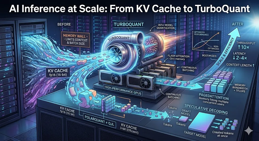
AI Inference at Scale: From KV Cache to TurboQuant — Making Your Models 10× Faster
In AI 11, we fine-tuned a custom model and deployed it on our own hardware. Ownership achieved. But Month 2 arrives and your self-hosted Llama-70B is processing 5,000 queries/day — and the RTX 4090 is running out of memory at 32K context. Users are queuing. Latency is climbing. You’re already thinking about a second GPU.
Before you buy more hardware, make the hardware you already have work 10× harder.
This is the inference optimization problem — and it’s where the real engineering happens after you’ve trained or selected a model. Training is a one-time cost. Inference is the cost you pay on every single query, forever. A 2× improvement in inference efficiency is equivalent to cutting your GPU fleet in half — or doubling your user capacity overnight.
TL;DR
Inference optimization is the difference between a 5,000/year one — for the same model, the same quality, the same users.
The Inference Optimization Stack:

  ┌──────────────────────────────────────────────────────────────┐
  │               AI Inference Optimization Stack                 │
  │                                                              │
  │  Model Quantization       KV Cache Compression               │
  │  (AI 11 → AI 12)         (NEW in AI 12)                     │
  │  ║                        ║                                  │
  │  What changes:            What changes:                      │
  │  Weight precision         Attention memory footprint         │
  │  16-bit → 4-bit           32-bit → 3-bit per KV element     │
  │                                                              │
  │  Speculative Decoding     Serving Infrastructure             │
  │  (NEW in AI 12)           (AI 11 → AI 12)                   │
  │  ║                        ║                                  │
  │  What changes:            What changes:                      │
  │  Generation strategy      Request batching & scheduling      │
  │  1 token → 5+ tokens     Static → continuous batching       │
  │                                                              │
  │  Combined effect: 5-10× throughput, 2-4× latency reduction  │
  └──────────────────────────────────────────────────────────────┘
Article Map
I — Problem Layer (where time and memory go)
- The Inference Cost Wall — Why inference dominates your AI budget
- GPU Memory Anatomy — Model weights vs. KV Cache vs. activations
- The KV Cache: Where Your Memory Actually Goes — The hidden bottleneck
II — Technique Layer (how to optimize) 4. Model Quantization for Inference — GPTQ, AWQ, GGUF: choosing the right format 5. KV Cache Compression — GQA, Sliding Window, and why KV is harder 6. TurboQuant Deep Dive — Google’s breakthrough: 3-bit KV with zero training 7. Speculative Decoding — Draft-verify: generating 5 tokens in the time of 1 8. Flash Attention — Making O(n²) bearable
III — Engineering Layer (production deployment) 9. Serving Infrastructure — vLLM, TensorRT-LLM, SGLang 10. Hardware Selection & Cost Engineering — GPU comparison, bandwidth math 11. Monitoring Inference Quality — Ensuring optimization doesn’t degrade output 12. Key Takeaways
1. The Inference Cost Wall
1.1 Training vs. Inference: Where the Money Goes
Every AI system has two cost phases. Most people obsess over the wrong one:
AI Cost Lifecycle:

  Training (one-time or periodic):
  ──────────────────────────────
  Fine-tune Llama-8B on 5,000 examples:
    Cloud GPU time: ~$50-200 (4 hours on A100)
    Data preparation: ~$4,000 (40 hours × $100/hr)
    Total: ~$4,200 (one-time)

  Inference (every query, forever):
  ─────────────────────────────────
  1,000 queries/day × 365 days × $0.03/query (self-hosted):
    Year 1: $10,950
    Year 2: $10,950
    Year 3: $10,950

  Ratio: Inference cost = 8× training cost by Year 3.
  At 10,000 queries/day: Inference = 80× training.

  ┌──────────────────────────────────────────────────────┐
  │  The Rule of Inference:                               │
  │                                                      │
  │  Training cost is fixed. Inference cost scales       │
  │  linearly with users. Every efficiency gain in       │
  │  inference multiplies across every query, every      │
  │  user, every day.                                    │
  │                                                      │
  │  A 2× faster inference = 50% cost reduction forever. │
  └──────────────────────────────────────────────────────┘
1.2 The Three Bottlenecks
Why LLM Inference Is Slow — The Three Bottlenecks:

  Bottleneck 1: Memory Bandwidth (THE dominant bottleneck)
  ────────────────────────────────────────────────────────
  LLM inference is memory-bound, not compute-bound.

  Why? During autoregressive generation, the model generates
  one token at a time. Each token requires reading the ENTIRE
  model's weights from VRAM — but only performs a tiny amount
  of computation per weight.

  RTX 4090: 1,008 GB/s memory bandwidth
  Llama-8B fp16: 16 GB model weights
  Time to read all weights once: 16 GB / 1,008 GB/s = 15.9 ms
  → Maximum theoretical speed: ~63 tokens/second
  → Actual: ~40-50 tokens/second (overhead)

  ⚠ This is at Batch Size = 1 (one user, sequential generation).
  At BS=1, you read 16 GB of weights to produce ONE token.
  At BS=32, the same 16 GB read produces 32 tokens — the weight
  read cost is amortized across the batch, and suddenly the GPU's
  82 TFLOPS of compute start to matter. This is why Continuous
  Batching (§9) is transformative for throughput.

  The GPU's 82 TFLOPS of compute power sits mostly idle at BS=1.
  This is the "arithmetic intensity" problem: too few FLOPs
  per byte loaded from memory.

  Bottleneck 2: KV Cache Memory (limits context + batch size)
  ────────────────────────────────────────────────────────────
  Each token's Key and Value vectors must be stored for ALL
  previous tokens in the sequence. At long contexts:

  Llama-70B, 128K context:
    KV Cache per sequence: ~40 GB  ← MORE than the model itself
    With batch size 8: 320 GB      ← Exceeds even H100 80GB

  This limits how many users you can serve simultaneously
  and how long their conversations can be.

  Bottleneck 3: Sequential Generation
  ────────────────────────────────────
  Autoregressive models generate ONE token at a time.
  Each token depends on the previous one.

  500-token response at 50 tokens/sec = 10 seconds.
  No amount of GPU parallelism helps — the dependency is
  fundamental to how language models work.

  (Speculative decoding §7 addresses this.)
🔧 Engineer’s Note: Before optimizing anything, identify which bottleneck dominates your workload. Short queries with large batches? You’re memory-bandwidth bound — quantize the model weights (§4). Long-context RAG with few concurrent users? You’re KV-cache bound — compress the cache (§5-6). Interactive chat needing low latency? You’re sequentiality-bound — use speculative decoding (§7). The wrong optimization applied to the wrong bottleneck wastes effort.
2. GPU Memory Anatomy: Where Your VRAM Actually Goes
2.1 The Four Consumers of VRAM
During inference, GPU memory is consumed by four components. Understanding their relative sizes is essential for choosing the right optimization:
VRAM Breakdown During Inference (Llama-3.1 8B, fp16):

  ┌──────────────────────────────────────────────────────┐
  │  Component           │ Size       │ % of Total       │
  ├──────────────────────┼────────────┼──────────────────┤
  │  Model Weights       │ 16.0 GB    │ 76%              │
  │  KV Cache (4K ctx)   │ 1.0 GB     │ 5%               │
  │  Activations         │ 0.5 GB     │ 2%               │
  │  Framework Overhead  │ 3.5 GB     │ 17%              │
  │                      │            │                  │
  │  Total               │ 21.0 GB    │ 100%             │
  └──────────────────────┴────────────┴──────────────────┘

  Same model at 128K context:
  ┌──────────────────────┬────────────┬──────────────────┐
  │  Model Weights       │ 16.0 GB    │ 38%              │
  │  KV Cache (128K ctx) │ 24.0 GB    │ 57%  ← DOMINANT  │
  │  Activations         │ 1.5 GB     │ 3%               │
  │  Framework Overhead  │ 0.5 GB     │ 2%               │
  │                      │            │                  │
  │  Total               │ 42.0 GB    │ Too big for 4090!│
  └──────────────────────┴────────────┴──────────────────┘

  The shift is dramatic:
  At short context → model weights dominate → quantize weights
  At long context  → KV cache dominates    → compress KV cache
2.2 The Memory Bandwidth Equation
Why Inference Speed = Memory Bandwidth ÷ Model Size:

  Tokens per second (theoretical max):

  tps = Memory Bandwidth (GB/s) ÷ Model Size (GB)

  ┌──────────────────────────────────────────────────────────┐
  │ Hardware        │ BW (GB/s) │ 8B fp16  │ 8B INT4  │ 70B │
  ├──────────────────────────────────────────────────────────┤
  │ RTX 4090        │ 1,008     │ 63 tps   │ 210 tps  │ N/A │
  │ Apple M4 Max    │ 546       │ 34 tps   │ 114 tps  │ 13  │
  │ H100 SXM        │ 3,350     │ 209 tps  │ 698 tps  │ 48  │
  │ 2× H100 NVLink  │ 6,700     │ 418 tps  │ 1,396tps │ 96  │
  └──────────────────────────────────────────────────────────┘

  Key insight: Quantizing from fp16 → INT4 = 4× smaller model
  = 4× less data to read from memory = ~3.3× faster inference

  This is why quantization is the single highest-ROI optimization:
  it directly reduces the bottleneck (bytes read per token).
🔧 Engineer’s Note: Memory bandwidth, not TFLOPS, determines your inference speed. The RTX 4090 has 82 TFLOPS of compute but only 1,008 GB/s of bandwidth. During token generation, the GPU spends 95% of its time waiting for data from VRAM and 5% computing. This is why the Apple M4 Max — with far fewer TFLOPS but unified memory architectures — can be surprisingly competitive for inference: lower bandwidth, but zero copy overhead between CPU and GPU memory.
3. The KV Cache: Where Your Memory Actually Goes
3.1 What Is the KV Cache? (Back to AI 00 §6.2)
In AI 00 §6.2, we covered Self-Attention: each token computes Query, Key, and Value vectors, and attention is calculated as:
During generation, the model produces tokens one at a time. For token 500, it needs the K and V vectors of all 499 previous tokens to compute attention. Without caching, it would recompute all 499 tokens’ K/V from scratch — on every single new token.
The KV Cache stores these vectors so they only need to be computed once:
KV Cache: Trading Memory for Speed

  Without KV Cache (naive):
    Token 1:   Compute K₁, V₁                    → 1 computation
    Token 2:   Recompute K₁, V₁, compute K₂, V₂  → 3 computations
    Token 3:   Recompute K₁, V₁, K₂, V₂, + K₃V₃ → 5 computations
    Token 500: Recompute all 499 previous + new   → 999 computations

    Total for 500 tokens: O(n²) computations → extremely slow

  With KV Cache (standard):
    Token 1:   Compute K₁, V₁, store in cache     → 1 computation
    Token 2:   Load K₁, V₁ from cache, compute K₂V₂, store → 1 new
    Token 3:   Load K₁V₁, K₂V₂ from cache, compute K₃V₃   → 1 new
    Token 500: Load 499 from cache, compute 1 new           → 1 new

    Total for 500 tokens: O(n) computations → 500× faster

    Cost: storing all those K,V vectors in VRAM
3.2 KV Cache Size Calculation
KV Cache Memory Formula:

  KV_size = 2 × n_layers × n_kv_heads × d_head × seq_len × precision_bytes

  For Llama-3.1 8B:
    n_layers   = 32
    n_kv_heads = 8  (GQA: 8 KV heads for 32 query heads)
    d_head     = 128
    seq_len    = varies
    precision  = 2 bytes (fp16)

  Per token: 2 × 32 × 8 × 128 × 2 = 131,072 bytes = 128 KB

  ┌──────────────────────────────────────────────────────┐
  │ Context Length │ KV Cache Size  │ % of Model (16GB)  │
  ├──────────────────────────────────────────────────────┤
  │ 1K tokens      │ 128 MB         │ 0.8%               │
  │ 4K tokens      │ 512 MB         │ 3.2%               │
  │ 32K tokens     │ 4 GB           │ 25%                │
  │ 128K tokens    │ 16 GB          │ 100% — same as     │
  │                │                │ the model itself!   │
  └──────────────────────────────────────────────────────┘

  For Llama-3.1 70B (MHA: 64 KV heads):
  ┌──────────────────────────────────────────────────────┐
  │ 4K tokens      │ 5 GB           │                    │
  │ 32K tokens     │ 40 GB          │ Exceeds single H100│
  │ 128K tokens    │ 160 GB         │ Requires 4× H100   │
  └──────────────────────────────────────────────────────┘

  Now multiply by batch size (concurrent users):
  8 users × 32K context × 70B model = 320 GB KV Cache alone
  + 140 GB model weights = 460 GB total → massive GPU cluster
3.3 Why KV Cache Compression Matters More Than Weight Quantization
The Crossover Point:

  Memory (GB)
  40 ┤
     │           ╱ KV Cache (grows with context)
  30 ┤         ╱
     │       ╱
  20 ┤─────╱──────── Model Weights (fixed after quantization)
     │   ╱
  10 ┤ ╱
     │╱
   0 ┼───────────────────── Context Length
     0    4K   16K  32K  64K  128K

  Below ~8K context: Model weights dominate.
    → Weight quantization (§4) is the highest ROI.

  Above ~16K context: KV cache dominates.
    → KV cache compression (§5-6) is the highest ROI.

  At 128K context: KV cache is 4-10× the model weights.
    → KV compression is ESSENTIAL, not optional.

  Modern RAG systems (AI 03) routinely inject 10K-50K tokens
  of context. This is squarely in KV-cache-dominant territory.
🔧 Engineer’s Note: If you’re serving a RAG application (AI 03) with long retrieved contexts, KV Cache compression will give you a bigger throughput gain than model quantization. Most teams quantize the model weights and stop there. They’ve optimized the smaller problem. The real bottleneck at long contexts is the KV Cache — and until recently, there wasn’t a good way to compress it without quality loss. TurboQuant (§6) changes this.
4. Model Quantization for Inference
4.1 From AI 11 to AI 12: Training-Time vs. Inference-Time Quantization
In AI 11 §4.3, we used QLoRA — 4-bit quantization for training. The base model was quantized to reduce VRAM during fine-tuning, while LoRA adapters trained in fp16.
AI 12 focuses on inference-time quantization: compressing the final model weights for faster, cheaper serving. The techniques are different:
Training-Time vs. Inference-Time Quantization:

  Training-Time (AI 11 QLoRA):
  ────────────────────────────
  Goal: Fit the model in VRAM during training
  Method: bitsandbytes NF4 on-the-fly dequantization
  Quality: Gradients computed in fp16 → no quality loss
  Output: fp16 LoRA adapters + fp16 merged model

  Inference-Time (AI 12):
  ───────────────────────
  Goal: Serve the model faster and cheaper
  Method: GPTQ, AWQ, or GGUF post-training quantization
  Quality: Small quality loss (typically <2% on benchmarks)
  Output: Quantized model file ready for deployment

  Typical workflow:
  1. Fine-tune with QLoRA (AI 11) → produces fp16 merged model
  2. Quantize for inference (AI 12) → produces INT4 serving model
  3. Deploy with vLLM or llama.cpp → serves queries at 3× speed
4.2 The Three Quantization Formats
Quantization Format Comparison:

  ┌────────────────────────────────────────────────────────────────┐
  │ Format │ Best For          │ Engine          │ Key Feature     │
  ├────────────────────────────────────────────────────────────────┤
  │ GGUF   │ CPU, Apple Silicon│ llama.cpp,      │ Layer offloading│
  │        │ Edge, local       │ Ollama, LM      │ (CPU+GPU split) │
  │        │                   │ Studio          │                 │
  ├────────────────────────────────────────────────────────────────┤
  │ AWQ    │ Production GPU    │ vLLM, TGI,      │ Activation-aware│
  │        │ High accuracy     │ SGLang          │ (protects key   │
  │        │                   │                 │  weights)       │
  ├────────────────────────────────────────────────────────────────┤
  │ GPTQ   │ High-throughput   │ ExLlamaV2,      │ Mature, fastest │
  │        │ GPU production    │ vLLM, AutoGPTQ  │ on NVIDIA       │
  └────────────────────────────────────────────────────────────────┘

  Decision tree:
  ├── Running locally / laptop / Mac? → GGUF
  ├── Production GPU server with vLLM? → AWQ (best accuracy)
  └── Maximum throughput on NVIDIA?    → GPTQ (fastest kernels)
4.3 GGUF: The Local Deployment Standard
GGUF (GPT-Generated Unified Format) is the standard for local and edge deployment. It supports flexible quantization levels and CPU/GPU hybrid execution:
# Quantizing a fine-tuned model to GGUF for Ollama deployment
# Step 1: Convert from HuggingFace to GGUF (using llama.cpp)

# Clone and build llama.cpp
# git clone https://github.com/ggerganov/llama.cpp
# cd llama.cpp && make -j

# Convert merged model to GGUF fp16 baseline
# python convert_hf_to_gguf.py \
#   ../models/financial-ai-merged/ \
#   --outfile financial-ai-f16.gguf \
#   --outtype f16

# Step 2: Quantize to target precision
# ./llama-quantize financial-ai-f16.gguf financial-ai-q4_k_m.gguf Q4_K_M
GGUF Quantization Levels (8B model):
┌──────────────────────────────────────────────────────────────┐
│ Quant │ Bits │ Size │ Quality │ Speed vs fp16 │
├──────────────────────────────────────────────────────────────┤
│ Q8_0 │ 8 │ 8.5 GB │ Near-lossless │ ~1.5× faster │
│ Q6_K │ 6 │ 6.1 GB │ Excellent │ ~2.0× faster │
│ Q5_K_M │ 5 │ 5.3 GB │ Very good │ ~2.5× faster │
│ Q4_K_M │ 4 │ 4.6 GB │ Good (default) │ ~3.0× faster │
│ Q3_K_M │ 3 │ 3.5 GB │ Acceptable │ ~3.5× faster │
│ Q2_K │ 2 │ 2.9 GB │ Degraded │ ~4.0× faster │
├──────────────────────────────────────────────────────────────┤
│ Recommended for domain AI: │
│ Q5_K_M or Q4_K_M — always validate with perplexity test │
│ (AI 11 §9.3) │
└──────────────────────────────────────────────────────────────┘4.4 AWQ: Activation-Aware Quantization for Production
AWQ (Activation-Aware Weight Quantization) is the highest-quality 4-bit format. Its key insight: not all weights matter equally. By observing which weights cause the largest activation magnitudes, AWQ protects the “salient” weights while aggressively quantizing the rest:
# AWQ quantization for production serving with vLLM
from awq import AutoAWQForCausalLM
from transformers import AutoTokenizer

# Load the fine-tuned fp16 model
model_path = "./models/financial-ai-merged"
quant_path = "./models/financial-ai-awq"

model = AutoAWQForCausalLM.from_pretrained(model_path)
tokenizer = AutoTokenizer.from_pretrained(model_path)

# AWQ quantization config
quant_config = {
    "zero_point": True,      # Include zero-point for better accuracy
    "q_group_size": 128,     # Quantize in groups of 128 weights
    "w_bit": 4,              # 4-bit quantization
}

# Load ~200 calibration samples from your domain
# Use YOUR data — not generic WikiText — for domain-specific protection
from datasets import load_dataset
dataset = load_dataset("your_org/financial_ifrs_qa", split="train[:200]")
calib_data = [example["text"] for example in dataset]

# Quantize — AWQ uses these to identify "salient" weights
model.quantize(
    tokenizer,
    quant_config    = quant_config,
    calib_data      = calib_data,
    # AWQ observes activations on your domain data to determine
    # which weights are critical and must retain higher precision
)

model.save_quantized(quant_path)
tokenizer.save_pretrained(quant_path)

# Deploy with vLLM (AI 11 §9)
# python -m vllm.entrypoints.openai.api_server \
#   --model ./models/financial-ai-awq \
#   --quantization awq \
#   --max-model-len 32768
AWQ vs Standard Quantization — Why Activation-Awareness Matters:
Standard INT4 quantization:
Treats all weights equally → compresses every weight to 4 bits
Result: some critical weights lose precision → quality degrades
AWQ:
Step 1: Run 200 calibration examples through the fp16 model
Step 2: Measure activation magnitudes (which weights matter most)
Step 3: Protect salient weights (keep more precision bits)
Step 4: Aggressively quantize non-salient weights
Result: same 4-bit average compression, but quality retained
Benchmark comparison (Llama-3.1 8B, MMLU):
fp16 baseline: 68.4%
Standard INT4: 66.1% (−2.3%)
AWQ INT4: 67.9% (−0.5%) ← 4× less quality loss
GPTQ INT4: 67.2% (−1.2%)🔧 Engineer’s Note: AWQ’s 200-sample calibration is not optional — it’s what makes AWQ better than GPTQ. Use calibration samples from your actual domain, not generic WikiText. For financial AI: use 200 representative IFRS queries. For code generation: use 200 representative code snippets. The calibration data tells AWQ which weights are critical for your use case. Generic calibration produces generic protection — domain-specific calibration produces domain-specific quality retention.
4.5 The Weight Problem Is Solved. The Context Problem Isn’t.
Model quantization solves the weight problem — and it solves it well. You’ve shrunk the 16 GB model to 4 GB, inference is 3× faster, and quality loss is under 1%. But it completely ignores the context problem.
At 128K context, your KV Cache is still ballooning to 24 GB — untouched by weight quantization, growing linearly with every token, and consuming 6× more memory than your beautifully quantized 4 GB model. You’ve optimized the fixed cost and left the variable cost unchecked.
To truly scale inference, we must compress the thing that weight quantization can’t reach: the KV Cache.
5. KV Cache Compression: The New Frontier
5.1 Why KV Cache Is Harder to Quantize Than Model Weights
Model weights are static — they’re fixed after training and the same for every query. You can spend hours carefully calibrating their quantization. KV Cache entries are dynamic — they’re generated on-the-fly during inference, unique to each user’s input, and must be quantized in real time:
Why KV Cache Quantization Is Harder:

  Model Weights:                    KV Cache:
  ──────────────                    ─────────
  Static (fixed after training)     Dynamic (new every query)
  Calibrate offline with 200+       Must quantize in real time
  examples, take your time          (microseconds per token)

  Distribution: well-studied,       Distribution: varies wildly
  smooth, predictable                by layer, head, and input

  Outliers: rare, manageable        Outliers: common, especially
                                    in early layers — one large
                                    value can destroy quantization
                                    for the entire channel

  The Outlier Problem:
  ┌──────────────────────────────────────────────────────┐
  │  Typical KV vector in Layer 2 (fp16):               │
  │  [0.12, 0.08, -0.15, 0.11, 42.7, 0.09, -0.13, ...] │
  │                        ↑                             │
  │                   Outlier channel                     │
  │                                                      │
  │  If you quantize to INT4 (range: -8 to +7):         │
  │  Scale = 42.7 / 7 = 6.1                             │
  │  0.12 / 6.1 = 0.02 → quantizes to 0 ← DESTROYED    │
  │  0.08 / 6.1 = 0.01 → quantizes to 0 ← DESTROYED    │
  │                                                      │
  │  One outlier ruins precision for ALL other values    │
  │  in that channel. This is called "activation sink."  │
  └──────────────────────────────────────────────────────┘
5.2 Architectural Solutions: GQA and Sliding Window
Before TurboQuant, the primary approaches to reducing KV Cache size were architectural — they require the model to be designed (or retrained) with smaller caches:
Grouped-Query Attention (GQA):

  Standard Multi-Head Attention (MHA):
    32 Query heads → 32 Key heads → 32 Value heads
    KV Cache per token: 32 × 2 × d_head × 2 bytes = 16 KB

  Grouped-Query Attention (GQA):
    32 Query heads → 8 Key heads → 8 Value heads
    KV Cache per token:  8 × 2 × d_head × 2 bytes = 4 KB (4× smaller!)

  How it works:
    Query heads are divided into groups. Each group of 4 query
    heads shares 1 Key head and 1 Value head.

    ┌──────────────────────────────────────────────────────┐
    │  MHA:  Q₁→K₁  Q₂→K₂  Q₃→K₃  Q₄→K₄  (4 KV pairs)  │
    │  GQA:  Q₁→K₁  Q₂→K₁  Q₃→K₁  Q₄→K₁  (1 KV pair!)  │
    │                                                      │
    │  4 queries share 1 key-value pair = 4× less KV VRAM │
    └──────────────────────────────────────────────────────┘

  Who uses it:
    Llama 3.1 8B:  32 Q heads, 8 KV heads (4:1 ratio)
    Llama 3.1 70B: 64 Q heads, 8 KV heads (8:1 ratio)
    Gemma 2/3:     All variants use GQA
    Mistral 7B:    32 Q heads, 8 KV heads

  Trade-off: <1% quality degradation vs MHA on most benchmarks.
  This is why modern open-source models universally adopt GQA —
  the quality cost is negligible, the memory savings are 4-8×.
Sliding Window Attention (Mistral):
Standard attention: every token attends to ALL previous tokens.
Token 10,000 attends to tokens 1-9,999 (huge KV cache)
Sliding window: each token attends to only the last W tokens.
Token 10,000 attends to tokens 5,953-9,999 (W=4,096)
KV Cache is capped at W entries, regardless of total length.
┌──────────────────────────────────────────────────────┐
│ Standard: │
│ [████████████████████████████████] all tokens │
│ KV Cache grows forever ↑ │
│ │
│ Sliding Window (W=4096): │
│ [ ████████████████████] last 4096 only │
│ Fixed KV Cache size ↑ │
└──────────────────────────────────────────────────────┘
Limitation: Information beyond W tokens is lost.
Mitigation: Interleaved layers — some layers use full attention,
others use sliding window. Gemma 3 and Mistral use this hybrid
approach to maintain long-range reasoning while capping memory.5.3 The Gap: Post-Training KV Compression
GQA and Sliding Window are powerful but require model architecture changes — you can’t retrofit them to an existing trained model. What if you’ve already fine-tuned a model (AI 11) and want to compress its KV Cache without retraining?
This is the gap that post-training KV Cache quantization fills. And until March 2026, every approach had the same problem: significant quality degradation at aggressive compression levels (below 4-bit).
Post-Training KV Compression — The State Before TurboQuant:

  Method             │ Bits │ Quality Loss │ Limitation
  ───────────────────┼──────┼──────────────┼──────────────────────
  Per-channel INT8   │ 8    │ Negligible   │ Only 2× compression
  Per-channel INT4   │ 4    │ 1-3%         │ Outlier sensitivity
  KVQuant (2024)     │ 2-4  │ 2-5%         │ Needs calibration data
  KIVI (2024)        │ 2    │ 3-8%         │ Per-channel tuning
  ───────────────────┼──────┼──────────────┼──────────────────────
  TurboQuant (2026)  │ ~3   │ <0.5%        │ None — plug and play
🔧 Engineer’s Note: GQA is the “free lunch” of KV Cache reduction — use models that have it. When selecting a base model for fine-tuning (AI 11 §3), always prefer GQA models (Llama 3.x, Gemma 2/3, Mistral) over MHA models. A Llama-3.1-8B with GQA has 4× smaller KV Cache than a hypothetical MHA variant — that’s 4× more concurrent users or 4× longer context on the same GPU, with no quality cost. This is a free optimization baked into the architecture.
6. TurboQuant Deep Dive
6.1 The Breakthrough: 3-Bit KV with Near-Zero Quality Loss
TurboQuant, published by Google Research at ICLR 2026, is a two-stage KV Cache compression pipeline that achieves ~3 bits per element with near-zero accuracy loss — and requires no retraining, no calibration data, and no model-specific tuning:
TurboQuant: What It Achieves

  ┌──────────────────────────────────────────────────────────────┐
  │  Before TurboQuant:                                          │
  │  KV Cache in fp16 (16 bits per element)                      │
  │  Llama-70B at 32K context: ~40 GB KV Cache                  │
  │                                                              │
  │  After TurboQuant:                                           │
  │  KV Cache at ~3 bits per element                             │
  │  Llama-70B at 32K context: ~7.5 GB KV Cache                 │
  │                                                              │
  │  Compression: 5.3×                                           │
  │  Quality loss: <0.5% on downstream benchmarks               │
  │  Retraining required: None                                   │
  │  Calibration data required: None                             │
  │                                                              │
  │  Attention speedup on H100: up to 8× for logit computation  │
  └──────────────────────────────────────────────────────────────┘

  Why this matters for your self-hosted model (AI 11):
  ├── That 70B model that needed 4× H100 at 128K context?
  │   Now runs on 1× H100.
  ├── Your 8B model on an RTX 4090 at 32K context?
  │   Now supports 5× more concurrent users.
  └── KV Cache is no longer the bottleneck — weights are again.
6.2 Stage 1: PolarQuant — Rotation + Polar Coordinates
The first stage solves the outlier problem (§5.1) through an elegant mathematical transformation:
PolarQuant — The Intuition:

  The Problem (recap):
    KV vectors have outlier channels that destroy uniform quantization.
    [0.12, 0.08, -0.15, 42.7, 0.09]  ← outlier ruins everything

  The Solution: Rotate the vector so outliers spread evenly.

  Step 1: Random Orthogonal Rotation
  ──────────────────────────────────
  Multiply each KV vector by a random orthogonal matrix R.

  v_rotated = R · v_original

  Why? An orthogonal rotation preserves all dot products
  (and therefore all attention scores — the math is invariant).
  But it SPREADS the energy of outlier channels across ALL
  dimensions uniformly.

  Before rotation: [0.12, 0.08, -0.15, 42.7, 0.09]
                                   ↑ One outlier = 99% of energy
  After rotation:  [8.53, -9.11, 7.94, -8.82, 8.70]
                    Energy distributed evenly ← quantization-friendly!

  Analogy: Imagine a spikey ball of clay. Before quantization,
  the spike pokes through the grid lines. If you roll it into
  a smooth sphere first (rotation), it fits neatly into any grid.

  Step 2: Polar Coordinate Transform
  ──────────────────────────────────
  Convert the rotated vector from Cartesian (x,y,z,...) to
  polar coordinates (radius r, angles θ₁, θ₂, ...).

  Why? After rotation, the angular distributions become smooth
  and predictable — ideal for uniform quantization.

  The radius (magnitude) is stored at higher precision (it's just
  one number per vector). The angles are quantized to ~3 bits each.

  Key advantage over traditional quantization:
  No per-group scale/zero-point constants needed.
  Traditional INT4 stores a scale + zero for every 128 weights
  → metadata overhead = ~0.5 bits per element.
  PolarQuant's metadata overhead = ~0 (the rotation matrix R
  is shared across the entire model, not per-group).
6.3 Stage 2: QJL — 1-Bit Error Correction
The second stage corrects the small residual error from PolarQuant using the Johnson-Lindenstrauss lemma:
QJL (Quantized Johnson-Lindenstrauss) — The Error Corrector:

  After PolarQuant, there's a small quantization error ε:
    v_quantized = v_original + ε

  QJL captures this error using a remarkable trick:

  Step 1: Project ε into a lower-dimensional space
  ─────────────────────────────────────────────────
  Multiply ε by a random Gaussian matrix G:
    projected = G · ε

  The Johnson-Lindenstrauss lemma guarantees that distances
  (and similarities) are approximately preserved even in
  the lower-dimensional space.

  Step 2: Store only the SIGN of each projected value
  ─────────────────────────────────────────────────────
  sign(projected) = +1 or -1 → exactly 1 bit per element

  This 1-bit sketch corrects the systematic bias of PolarQuant.

  Total bits per KV element:
  ├── PolarQuant:    ~2 bits (quantized angles)
  ├── QJL:           ~1 bit (sign sketch)
  └── Total:         ~3 bits per element

  Compression ratio: 16 bits → ~3 bits = 5.3× reduction

  The Two Stages Complement Each Other:
  ┌──────────────────────────────────────────────────────┐
  │  PolarQuant alone:  ~2 bits, 0.8-1.2% quality loss  │
  │  QJL alone:         N/A (needs a base quantization)  │
  │  PolarQuant + QJL:  ~3 bits, <0.5% quality loss     │
  │                                                      │
  │  The 1-bit error correction cuts the remaining       │
  │  quality loss by 50-70% — trivial memory cost for    │
  │  significant quality recovery.                       │
  └──────────────────────────────────────────────────────┘
6.4 Why TurboQuant Is a Breakthrough (Not Just Another Paper)
What Makes TurboQuant Different from Previous KV Compression:

  Property          │ Previous Methods │ TurboQuant
  ──────────────────┼──────────────────┼──────────────────
  Retraining        │ Often required   │ None
  Calibration data  │ Usually required │ None
  Model-specific    │ Yes (per-model)  │ Model-agnostic
  Online (real-time)│ Some offline     │ Fully online
  Quality at 3-bit  │ 2-8% degradation │ <0.5% degradation

  The key: TurboQuant is plug-and-play.

  Previous methods: "Spend 2 days calibrating, fine-tune
  the quantization parameters for your specific model,
  run 1,000 examples through the pipeline, hope it generalizes."

  TurboQuant: "Enable it. Done."

  This is the difference between a research technique and
  a production tool. TurboQuant works on any Transformer
  model — Llama, Mistral, Gemma, GPT — without modification.

  Edge AI implication:
  With KV Cache at ~3 bits, a Llama-3.1 8B at 128K context
  needs only ~3 GB of KV memory (vs 16 GB in fp16).
  Combined with GGUF Q4_K_M weights (§4.3): total ~7.6 GB.
  This fits comfortably in unified-memory devices — high-end
  smartphones (iPhone 16 Pro: 8 GB), Raspberry Pi 5 (8 GB),
  or any laptop. Long-context on-device AI becomes real.
# TurboQuant integration (pseudocode — API varies by framework)
# As of April 2026, integration is available in vLLM and HuggingFace
# Option 1: vLLM with TurboQuant KV compression
# python -m vllm.entrypoints.openai.api_server \
# --model meta-llama/Meta-Llama-3.1-70B-Instruct \
# --kv-cache-dtype turbo_fp3 \ # Enable TurboQuant
# --max-model-len 131072 \ # 128K context — now fits!
# --tensor-parallel-size 2 # 2× H100 instead of 4×
# Option 2: HuggingFace Transformers (research/prototyping)
from transformers import AutoModelForCausalLM, TurboQuantConfig
turbo_config = TurboQuantConfig(
kv_bits = 3, # ~3 bits per KV element
polar_rotation = "random", # Random orthogonal rotation
qjl_correction = True, # Enable 1-bit error correction
)
model = AutoModelForCausalLM.from_pretrained(
"meta-llama/Meta-Llama-3.1-70B-Instruct",
device_map = "auto",
torch_dtype = "auto",
kv_cache_config = turbo_config, # Plug-and-play
)
# KV Cache now uses ~3 bits per element instead of 16
# 128K context KV Cache: 160 GB → ~30 GB (70B model)
# No retraining. No calibration. Just enable it.🔧 Engineer’s Note: TurboQuant’s real-world impact extends beyond memory savings to attention computation speed. Because the compressed KV Cache is smaller, the attention logit computation (Q·K^T from AI 00 §6.2) reads fewer bytes from memory — up to 8× fewer on H100. This directly translates to faster Time-to-First-Token (TTFT) for long-context queries. For RAG workloads (AI 03) where you inject 20K-50K tokens of retrieved context, the TTFT improvement alone can halve user-perceived latency — before you even consider the memory savings that enable larger batch sizes.
6.5 The Financial Impact: A “DeepSeek Moment”?
When Google published TurboQuant in March 2026, it triggered an immediate reaction in financial markets — semiconductor stocks (Micron, Samsung, SK Hynix) sold off on fears that software-based memory compression would reduce demand for physical memory chips.
The Market Reaction and Jevons Paradox:

  Fear: "If AI needs 5× less memory, GPU/HBM demand drops 5×."

  Reality: Jevons Paradox — efficiency increases TOTAL usage.

  ┌──────────────────────────────────────────────────────────┐
  │  Before TurboQuant:                                      │
  │  70B model at 128K context → needs 4× H100 (320 GB)     │
  │  Most teams: "We can't afford that. Use 8K context."     │
  │                                                          │
  │  After TurboQuant:                                       │
  │  70B model at 128K context → needs 1× H100 (80 GB)      │
  │  Most teams: "We can finally do 128K! And let's try 1M!" │
  │                                                          │
  │  Net effect: MORE GPU demand, not less.                  │
  │  Lower per-query cost → more queries become viable       │
  │  → total compute consumption increases.                  │
  │                                                          │
  │  Historical precedent:                                   │
  │  DeepSeek-V3 (Jan 2025): "Cheaper training!" → More      │
  │  teams started training custom models → GPU demand rose. │
  └──────────────────────────────────────────────────────────┘
🔧 Engineer’s Note: For your self-hosted models (AI 11), TurboQuant shifts the ROI calculation dramatically. The break-even analysis in AI 11 §10 assumed fp16 KV Cache — meaning long-context workloads required expensive multi-GPU setups. With TurboQuant, the self-hosting threshold drops: workloads that previously needed 2× H100 now fit on 1× RTX 4090. Re-run the break-even calculator from AI 11 §10.1 with 5× less KV memory — you’ll find the crossover point moves from 500 queries/day to around 200 queries/day.
7. Speculative Decoding: Breaking the Sequential Bottleneck
7.1 The Problem: One Token at a Time
In §1.2 Bottleneck 3, we identified the fundamental limitation: autoregressive models generate tokens sequentially. Token N+1 depends on token N. No parallelism possible.
Or is there?
The Speculative Decoding Insight:

  Standard autoregressive generation:
    Token 1 → Token 2 → Token 3 → Token 4 → Token 5
    Each step: full model forward pass (~15ms for 8B on 4090)
    5 tokens: 5 × 15ms = 75ms

  Speculative decoding:
    Draft model (fast, small) GUESSES tokens 2-5 in parallel
    Target model (accurate, large) VERIFIES all 4 guesses at once

    Step 1: Draft model generates 4 candidate tokens (~1ms each)
    Step 2: Target model verifies all 4 in ONE forward pass (~15ms)

    If 3 of 4 guesses are accepted: 4 tokens in ~19ms (vs 60ms)
    Speedup: ~3× for the same output quality

  Why does verification take the same time as generation?
  ──────────────────────────────────────────────────────
  Generating 1 token = read all model weights once.
  Verifying 4 tokens  = read all model weights once.

  Remember: the bottleneck is memory bandwidth (§1.2).
  Whether you generate 1 or verify 4, you read the same
  16 GB of weights. The compute for 4 tokens is trivial
  compared to the memory read.

  This is the most elegant exploitation of the
  memory-bandwidth bottleneck in modern AI engineering.
7.2 Draft-Target Architecture
Speculative Decoding Pipeline:

  ┌─────────────────────────────────────────────────────────┐
  │                                                         │
  │  Draft Model (Llama-3.2 1B)     Target Model (Llama 8B) │
  │  Fast: ~1ms per token           Slow: ~15ms per token   │
  │  Quality: OK (70% match)        Quality: Production     │
  │                                                         │
  │  Step 1: Draft generates K=5 candidate tokens           │
  │  ┌───────────────────────────────────────┐              │
  │  │ "The revenue grew" → [by, 15, %, in, Q3]            │
  │  └───────────────────────────────────────┘              │
  │  Time: 5 × 1ms = 5ms                                   │
  │                                                         │
  │  Step 2: Target verifies ALL 5 candidates at once       │
  │  ┌───────────────────────────────────────┐              │
  │  │ Token 1: "by"  → P=0.92 ✅ Accept     │              │
  │  │ Token 2: "15"  → P=0.87 ✅ Accept     │              │
  │  │ Token 3: "%"   → P=0.95 ✅ Accept     │              │
  │  │ Token 4: "in"  → P=0.91 ✅ Accept     │              │
  │  │ Token 5: "Q3"  → P=0.34 ❌ Reject     │              │
  │  │          "the" → P=0.78 (resample)    │              │
  │  └───────────────────────────────────────┘              │
  │  Time: 15ms (one forward pass, regardless of K)         │
  │                                                         │
  │  Result: 5 tokens in 20ms instead of 5 × 15ms = 75ms   │
  │  Speedup: 3.75× (with 80% acceptance rate)              │
  │                                                         │
  │  Critical property: OUTPUT IS MATHEMATICALLY IDENTICAL  │
  │  to standard generation. Rejected tokens are resampled  │
  │  from the target model's distribution. Zero quality loss.│
  └─────────────────────────────────────────────────────────┘
7.3 Choosing a Draft Model
Draft Model Selection Guide:

  The acceptance rate determines your speedup:

  Acceptance rate 90%: ~3.5× speedup (ideal)
  Acceptance rate 70%: ~2.5× speedup (typical)
  Acceptance rate 50%: ~1.5× speedup (marginal)
  Acceptance rate 30%: ~1.1× speedup (not worth the overhead)

  ┌──────────────────────────────────────────────────────────┐
  │ Target Model      │ Recommended Draft  │ Expected Match  │
  ├──────────────────────────────────────────────────────────┤
  │ Llama-3.1 70B     │ Llama-3.2 1B       │ 65-75%          │
  │ Llama-3.1 8B      │ Llama-3.2 1B       │ 70-80%          │
  │ Mistral 7B        │ Mistral 0.1B draft │ 75-85%          │
  │ Your fine-tuned 8B│ Base 1B from same   │ 60-75%          │
  │                   │ model family        │                 │
  └──────────────────────────────────────────────────────────┘

  Rules of thumb:
  ├── Same model family (Llama draft for Llama target) = highest match
  ├── Draft should be 5-10× smaller than target
  ├── Fine-tuned target + generic draft = lower acceptance
  │   → Consider distilling (AI 11 §6) a draft model too
  └── Domain-specific text has higher acceptance than creative text
      (financial reports are more predictable than poetry)
7.4 Beyond Draft Models: EAGLE and Medusa
Advanced Speculative Decoding (2025-2026):

  Method 1: EAGLE-3 (Feature-Level Speculation)
  ──────────────────────────────────────────────
  Instead of a separate draft model, EAGLE adds a lightweight
  prediction head that speculates from the target model's own
  hidden states. No separate model to load or manage.

  Advantage: Higher acceptance rate (uses richer features)
  Disadvantage: Requires model-specific training of the head

  Method 2: Medusa (Multi-Head Speculation)
  ─────────────────────────────────────────
  Adds multiple prediction heads to the target model,
  each predicting a different future token position.

  Head 1 predicts token N+1
  Head 2 predicts token N+2
  Head 3 predicts token N+3

  All heads run in parallel during one forward pass.
  Verification uses a tree structure to find the longest
  valid sequence.

  Method 3: Native Multi-Token Prediction (2026)
  ──────────────────────────────────────────────
  The emerging approach: train the model itself to predict
  multiple tokens per forward pass. No auxiliary model,
  no extra heads. The model natively outputs 3-5 tokens.

  Status: Research stage, but ~3× speedups demonstrated.
  This may eventually make speculative decoding obsolete
  by solving the problem at the architecture level.
# Speculative decoding with vLLM (production-ready)
# python -m vllm.entrypoints.openai.api_server \
# --model meta-llama/Meta-Llama-3.1-8B-Instruct \
# --speculative-model meta-llama/Llama-3.2-1B-Instruct \
# --num-speculative-tokens 5 \
# --max-model-len 32768
# Client code — completely transparent to the application
from openai import OpenAI
client = OpenAI(base_url="http://localhost:8000/v1", api_key="FAKE")
# The response is IDENTICAL to non-speculative generation
# but arrives 2-3× faster
response = client.chat.completions.create(
model = "meta-llama/Meta-Llama-3.1-8B-Instruct",
messages = [
{"role": "system", "content": "You are a CPA specializing in IFRS."},
{"role": "user", "content": "Classify this transaction..."},
],
stream = True, # Streaming works normally
)
# Monitoring: check acceptance rate in vLLM metrics
# curl http://localhost:8000/metrics | grep speculative
# vllm:spec_decode_acceptance_rate 0.78 ← 78% acceptance = good🔧 Engineer’s Note: Speculative decoding is the only optimization in this article that improves latency without any quality trade-off, and it’s completely transparent to your application code. The API response is mathematically identical — the client doesn’t know (or care) that speculative decoding is happening. For real-time financial AI (AI 08) where users wait for classification results, a 2-3× latency reduction from speculative decoding stacks multiplicatively with quantization speedups. A model that was 50 tokens/sec becomes 150 tokens/sec with INT4 quantization + speculative decoding — no quality loss.
8. Flash Attention: The IO-Aware Algorithm
8.1 The Memory Wall Inside Self-Attention
In AI 00 §6.1, we noted that Self-Attention has O(n²) complexity. But the naive implementation has an even bigger problem: it materializes the full n×n attention matrix in GPU memory — reading and writing it repeatedly between GPU SRAM (fast, tiny) and HBM (slow, large).
The standard three-step pipeline looks clean on paper:
But each arrow hides a devastating round-trip to slow HBM memory:
The IO Problem in Standard Attention:

  Standard implementation (naive):

  Step 1: Compute S = Q·Kᵀ               → Write n×n matrix to HBM
  Step 2: Compute P = softmax(S/√dₖ)     → Read S from HBM, write P to HBM
  Step 3: Compute O = P·V                 → Read P from HBM, write O to HBM

  Total HBM reads/writes: 3 × n² (for each of S, P, O)

  GPU memory hierarchy:
  ┌──────────────────────────────────────────────────────┐
  │  SRAM (on-chip):  ~20 MB   │ ~19 TB/s bandwidth    │
  │  HBM (off-chip):  80 GB    │ ~3.35 TB/s bandwidth  │
  └──────────────────────────────────────────────────────┘

  The SRAM is 5.7× faster but 4,000× smaller.
  Standard attention keeps bouncing data between them.

  At 128K context: n² = 16 billion elements
  Materializing the attention matrix = 32 GB in fp16
  → Exceeds the ENTIRE HBM of many GPUs just for one layer!
8.2 Flash Attention: Tiling + Online Softmax
Flash Attention (Dao et al., 2022) restructures the computation to never materialize the full n×n matrix. Instead, it processes attention in tiles that fit entirely in SRAM:
Flash Attention — The Key Insight:

  Instead of: Compute FULL Q·Kᵀ → softmax → multiply by V

  Do: Process in TILES that fit in SRAM

  ┌──────────────────────────────────────────────────────┐
  │  For each tile of Q (say, tokens 0-127):             │
  │    For each tile of K,V (say, tokens 0-127):         │
  │      1. Load Q_tile, K_tile, V_tile into SRAM        │
  │      2. Compute local attention: S_tile = Q_tile·K_tileᵀ│
  │      3. Apply ONLINE softmax (no need for full row)  │
  │      4. Accumulate O_tile = softmax_tile · V_tile    │
  │      5. Write only the accumulated O_tile to HBM     │
  │                                                      │
  │  The n×n matrix NEVER exists in HBM.                 │
  │  Only the final output O (n × d) is written.         │
  └──────────────────────────────────────────────────────┘

  "Online softmax" is the mathematical trick that makes this
  possible. Standard softmax needs the max of the entire row
  before computing. Online softmax maintains a running max
  and rescales accumulated values on-the-fly — no need to
  see all elements first.

  Result:
  ├── Memory: O(n) instead of O(n²) — no attention matrix stored
  ├── Speed: 2-4× faster (fewer HBM reads/writes)
  └── Exact: mathematically identical output (not approximate)
8.3 Flash Attention Evolution
Flash Attention Versions:

  FlashAttention-1 (2022):
    2-4× speedup, O(n) memory. Foundational IO-aware approach.

  FlashAttention-2 (2023):
    Better parallelism, ~2× faster than FA-1 on A100.
    Better sequence of operations to reduce synchronization.

  FlashAttention-3 (2024-2025):
    Optimized for H100 Hopper architecture specifically.
    Exploits: async Tensor Cores, TMA, warp specialization.
    Supports FP8 with 2.6× less numerical error than baseline.
    Reaches 75% of H100 theoretical FLOPS (FP16/BF16).
    1.5-2× faster than FA-2 on H100.

  Status (2026):
    FA-3 is the standard. Integrated into vLLM, HuggingFace,
    TensorRT-LLM. Enabled by default in most frameworks.

    If you're running on H100: you're using FA-3.
    If you're running on A100/4090: you're using FA-2.
    If you're not using Flash Attention: you're leaving
    2-4× performance on the table.
🔧 Engineer’s Note: Flash Attention is not optional — it’s the baseline. Every optimization in this article (quantization, KV compression, speculative decoding) builds on top of Flash Attention. If your serving framework doesn’t have it enabled, fix that first before pursuing anything else. It’s a free 2-4× speedup with zero quality loss and zero configuration beyond
pip install flash-attn. In vLLM, it’s enabled automatically when available.
9. Serving Infrastructure: vLLM, TensorRT-LLM, SGLang
9.1 Why the Serving Framework Matters More Than the Model
You’ve quantized your model (§4), compressed your KV Cache (§6), enabled speculative decoding (§7), and Flash Attention is running (§8). But if your serving framework handles requests naively — one user at a time, waiting for each to finish — you’re wasting 90% of your GPU’s capacity.
The serving framework is the orchestrator. It determines how many users your GPU can serve simultaneously.
9.2 The Revolution: Continuous Batching
Remember the batch-size annotation from §1.2? At BS=1, you read 16 GB of weights to produce one token. At BS=32, the same 16 GB read produces 32 tokens. Batching is the most powerful throughput multiplier in inference.
But traditional static batching has a fatal flaw:
Static Batching vs. Continuous Batching:

  Static Batching (naive):
  ────────────────────────
  Wait until B requests arrive, process them together,
  return ALL results, then accept the next batch.

  Problem: different requests have different output lengths.

  User A: "What is IFRS 16?" → 50 tokens  (done in 1 second)
  User B: "Explain all IFRS standards" → 500 tokens (10 seconds)

  Static: User A waits 10 seconds (until B finishes).
  GPU sits idle for 9 seconds on User A's slot.

  ┌──────────────────────────────────────────┐
  │ Time:  0s─────────5s──────────10s        │
  │ A:     [████░░░░░░░░░░░░░░░░░] idle wait │
  │ B:     [████████████████████████████████] │
  │        ↑ Both start    ↑ Both end         │
  │        GPU utilization: ~50%              │
  └──────────────────────────────────────────┘

  Continuous Batching (vLLM):
  ──────────────────────────
  As soon as a request finishes, its slot is immediately
  filled by the next waiting request. No waiting.

  ┌──────────────────────────────────────────┐
  │ Time:  0s────1s───2s───5s────10s         │
  │ A:     [████]                             │
  │ C:          [████████]     ← fills A's slot│
  │ D:                   [████████████]       │
  │ B:     [████████████████████████████████] │
  │        GPU utilization: ~95%              │
  └──────────────────────────────────────────┘

  Same GPU, same model, same quality:
  Static batching:     100 requests/minute
  Continuous batching: 300-500 requests/minute (3-5× more)
9.3 PagedAttention: Virtual Memory for KV Cache
vLLM’s second breakthrough (besides continuous batching) is PagedAttention — applying the operating system’s virtual memory concept to KV Cache management:
PagedAttention — The OS Analogy:

  Without PagedAttention (naive):
    Each request pre-allocates KV Cache for max_seq_len.
    Request asks for 4K context → allocate 4K × 128KB = 512 MB
    Request actually uses 500 tokens → 62 MB used, 450 MB wasted

    Waste: ~90% of pre-allocated KV memory is unused.
    With 8 concurrent users: 4 GB total, 3.6 GB wasted.

  With PagedAttention (vLLM):
    KV Cache is divided into fixed-size "pages" (blocks).
    Memory is allocated page-by-page as tokens are generated.

    Like OS virtual memory:
    ├── Physical pages are allocated on demand (no pre-allocation)
    ├── Non-contiguous pages are linked via a page table
    ├── Freed pages are recycled immediately for new requests
    └── Near-zero internal fragmentation

    Same 8 users, 500 tokens each:
    Actually used: 500 MB (vs 4 GB pre-allocated)

    Result: 3-5× more concurrent users on the same GPU.
9.4 Serving Framework Comparison
Inference Serving Frameworks (2026):

  ┌────────────────────────────────────────────────────────────────┐
  │ Framework     │ Key Feature          │ Best For                │
  ├────────────────────────────────────────────────────────────────┤
  │ vLLM          │ PagedAttention,      │ General production      │
  │               │ continuous batching, │ serving. Best ecosystem │
  │               │ LoRA hot-swap,       │ and community.          │
  │               │ speculative decode   │ OpenAI-compatible API.  │
  ├────────────────────────────────────────────────────────────────┤
  │ TensorRT-LLM  │ NVIDIA kernel        │ Maximum throughput on   │
  │               │ optimization,        │ NVIDIA GPUs. Harder     │
  │               │ FP8, in-flight       │ to set up, best raw     │
  │               │ batching             │ performance.            │
  ├────────────────────────────────────────────────────────────────┤
  │ SGLang        │ RadixAttention,      │ Complex multi-turn      │
  │               │ prefix caching,      │ and branching prompts.  │
  │               │ structured output    │ Excellent for agents.   │
  ├────────────────────────────────────────────────────────────────┤
  │ llama.cpp     │ CPU/hybrid, GGUF,    │ Local deployment,       │
  │ (+ Ollama)    │ minimal dependencies │ edge, development.      │
  │               │                      │ Not for production      │
  │               │                      │ multi-user serving.     │
  └────────────────────────────────────────────────────────────────┘

  Decision tree:
  ├── Production multi-user API? → vLLM (default choice)
  ├── Maximum NVIDIA throughput? → TensorRT-LLM
  ├── Complex agent workflows?   → SGLang
  └── Local dev / single user?   → Ollama (llama.cpp)
# Production vLLM deployment with ALL optimizations from this article
# This single command enables: quantization + KV compression +
# speculative decoding + continuous batching + PagedAttention
# python -m vllm.entrypoints.openai.api_server \
# --model ./models/financial-ai-awq \ # AWQ quantized (§4.4)
# --quantization awq \ # Enable AWQ kernels
# --kv-cache-dtype turbo_fp3 \ # TurboQuant KV (§6)
# --speculative-model meta-llama/Llama-3.2-1B-Instruct \ # Spec decode (§7)
# --num-speculative-tokens 5 \
# --max-model-len 65536 \ # 64K context
# --enable-prefix-caching \ # Cache common prefixes
# --max-num-seqs 64 \ # Up to 64 concurrent users
# --gpu-memory-utilization 0.92 # Use 92% of VRAM
# Combined effect on Llama-8B, RTX 4090:
# Baseline (fp16, no optimization): ~40 tps, 1 user, 4K context
# With ALL optimizations: ~150 tps, 32 users, 64K context
# Throughput improvement: ~120× (40 → 4,800 total tps)🔧 Engineer’s Note: vLLM is the “PostgreSQL of LLM serving” — the default choice that’s good enough for 95% of production workloads. Unless you have a specific reason to use TensorRT-LLM (absolute maximum throughput) or SGLang (complex agent routing), start with vLLM. Its OpenAI-compatible API means your application from AI 08 works unchanged — just point the
base_urlfrom the cloud API to your local vLLM server. Migration from API to self-hosted becomes a one-line config change.
10. Hardware Selection & Cost Engineering
10.1 The Hardware Landscape for Inference
GPU Comparison for LLM Inference (2026):

  ┌────────────────────────────────────────────────────────────────────┐
  │ GPU            │ VRAM  │ BW (GB/s)│ Price    │ Best For           │
  ├────────────────────────────────────────────────────────────────────┤
  │ RTX 4090       │ 24 GB │ 1,008   │ $1,600   │ 8B models, dev,    │
  │                │       │         │          │ small production    │
  ├────────────────────────────────────────────────────────────────────┤
  │ RTX 5090       │ 32 GB │ 1,792   │ $2,000   │ 8B-14B models,     │
  │                │       │         │          │ more headroom       │
  ├────────────────────────────────────────────────────────────────────┤
  │ Apple M4 Max   │ 128GB │ 546     │ $3,500   │ 70B local dev,     │
  │ (unified)      │       │         │(laptop)  │ prototyping         │
  ├────────────────────────────────────────────────────────────────────┤
  │ A100 80GB      │ 80 GB │ 2,039   │ $1.50/hr │ Cloud training +   │
  │ (cloud)        │       │         │          │ medium inference    │
  ├────────────────────────────────────────────────────────────────────┤
  │ H100 SXM       │ 80 GB │ 3,350   │ $2.50/hr │ Production 70B,    │
  │ (cloud)        │       │         │          │ highest throughput  │
  ├────────────────────────────────────────────────────────────────────┤
  │ 2× RTX 4090    │ 48 GB │ 2,016   │ $3,200   │ 70B INT4 on-prem,  │
  │ (NVLink n/a)   │       │(no link)│          │ requires TP split   │
  └────────────────────────────────────────────────────────────────────┘

  The bandwidth-per-dollar champion:
  RTX 4090: 1,008 GB/s ÷ $1,600 = 0.63 GB/s per dollar
  H100 SXM: 3,350 GB/s ÷ ~$30,000 = 0.11 GB/s per dollar

  The 4090 is 5.7× more cost-efficient per bandwidth dollar.
  This is why self-hosting on consumer GPUs (AI 11 §10) is so
  compelling for small-to-medium workloads.
10.2 Model-to-Hardware Fit
What Can You Run Where? (With AI 12 Optimizations)

  ┌──────────────────────────────────────────────────────────────┐
  │ Model        │ Precision │ VRAM Needed │ Hardware            │
  ├──────────────────────────────────────────────────────────────┤
  │ Llama 8B     │ INT4+TQ   │ ~6 GB      │ RTX 3060 12GB       │
  │ Llama 8B     │ INT4+TQ   │ ~6 GB      │ Apple M2 16GB       │
  │ Phi-4 14B    │ INT4+TQ   │ ~10 GB     │ RTX 4090 24GB       │
  │ Llama 70B    │ INT4+TQ   │ ~42 GB     │ 2× RTX 4090         │
  │ Llama 70B    │ INT4+TQ   │ ~42 GB     │ Apple M4 Max 128GB  │
  │ Llama 70B    │ INT4+TQ   │ ~42 GB     │ 1× H100 80GB        │
  │ Llama 405B   │ INT4+TQ   │ ~230 GB    │ 4× H100 (TP=4)      │
  └──────────────────────────────────────────────────────────────┘

  TQ = TurboQuant KV compression. Impact:
  Context at 32K on Llama 70B, 1× H100:
    Without TQ: model (35GB) + KV (40GB) = 75GB → barely fits
    With TQ:    model (35GB) + KV (7.5GB) = 42.5GB → room for
                batch size 4-5, or expand to 128K context
10.3 Updated ROI with AI 12 Optimizations
AI 11 §10 ROI Updated with AI 12 Optimizations:

  Original AI 11 calculation (fp16, no optimizations):
    1,000 queries/day, Llama-8B
    Self-hosted cost: $150/month (RTX 4090 server amortized)
    Break-even vs API: 9.4 months

  With AI 12 optimizations (INT4 + TurboQuant + spec decode):
    Same 1,000 queries/day, same Llama-8B
    Throughput: 3-5× higher → same GPU serves 3,000-5,000/day
    Context capacity: 4× longer → serves RAG workloads too

    Revised economics:
    ├── Same $150/month hardware cost
    ├── But now serving 3,000-5,000 queries/day (not 1,000)
    ├── Effective cost per query: $0.001 (vs $0.005 before)
    └── Break-even vs API: 3.1 months (vs 9.4)

  At 10,000 queries/day with optimizations:
    Single 4090 handles it (previously needed 2-3 GPUs)
    Break-even: 2 weeks
    Year 3 savings: $380,000+

  The optimization stack doesn't just save money —
  it moves the self-hosting threshold down dramatically.
  Workloads that couldn't justify self-hosting in AI 11
  now have clear ROI with AI 12's techniques.
🔧 Engineer’s Note: Buy bandwidth, not TFLOPS. When choosing inference hardware, rank by memory bandwidth per dollar, not by TFLOPS. The RTX 4090 and Apple M4 Max are the best consumer-grade inference machines precisely because they offer the most bandwidth per dollar. The H100 wins on absolute throughput (3.35 TB/s) but costs 20× more. For most self-hosted deployments (AI 11), 1-2× RTX 4090 with all AI 12 optimizations will outperform what teams were doing with 4× A100 just 18 months ago.
11. Monitoring Inference Quality
11.1 The Optimization-Quality Tradeoff
Every optimization in this article trades something for speed. Most trade-offs are tiny — but they compound. You must monitor quality continuously to ensure the stack of optimizations doesn’t silently degrade your domain accuracy:
Optimization Quality Impact — The Compound Risk:

  Optimization              │ Individual Loss │ Cumulative
  ──────────────────────────┼─────────────────┼──────────────
  AWQ INT4 weight quant     │ ~0.5%           │ 0.5%
  TurboQuant KV (3-bit)     │ ~0.3%           │ 0.8%
  Speculative decoding      │ 0% (exact)      │ 0.8%
  Flash Attention            │ 0% (exact)      │ 0.8%
  ──────────────────────────┼─────────────────┼──────────────
  Total stack               │                 │ ~0.8%

  0.8% on general benchmarks is negligible.
  But domain-specific degradation can be larger:

  General MMLU:           68.4% → 67.6%  (−0.8% — fine)
  IFRS classification:   94.2% → 91.1%  (−3.1% — concerning)

  Domain terminology (AI 11 §9.3) is where degradation hides.
  General benchmarks won't catch it. Domain evals will.
11.2 Production Monitoring Metrics
# Monitoring stack for optimized inference
# Connect to your eval pipeline from AI 09

INFERENCE_METRICS = {
    # Performance metrics (§1.2 bottlenecks)
    "ttft_ms":              "Time to first token (ms)",
    "tbt_ms":               "Time between tokens (ms)",
    "tokens_per_second":    "Generation throughput",
    "queue_depth":          "Pending requests",

    # Quality metrics (AI 09)
    "domain_ppl":           "Perplexity on domain test set",
    "judge_score_avg":      "LLM-as-Judge average (daily sample)",
    "faithfulness":         "RAGAS faithfulness (for RAG queries)",

    # Speculative decoding (§7)
    "spec_acceptance_rate": "Draft token acceptance rate",

    # Resource metrics
    "gpu_memory_used_gb":   "Current VRAM consumption",
    "kv_cache_usage_pct":   "KV Cache utilization %",
    "batch_size_avg":       "Average concurrent batch size",
}

# Alert thresholds
ALERTS = {
    "domain_ppl":           {"warn": 1.15, "critical": 1.30},
    # 15% PPL increase = warn, 30% = critical (AI 11 §9.3)

    "spec_acceptance_rate": {"warn": 0.50, "critical": 0.30},
    # Below 50% acceptance, speculative decoding hurts more than helps

    "ttft_ms":              {"warn": 2000, "critical": 5000},
    # >2s TTFT for interactive use is degraded UX

    "kv_cache_usage_pct":   {"warn": 0.85, "critical": 0.95},
    # Above 95% KV usage, new requests will be queued or dropped
}
The Inference Quality Dashboard:
┌──────────────────────────────────────────────────────────┐
│ Inference Quality Dashboard │
│ │
│ Domain PPL: 3.89 ✅ (baseline: 3.42, +13.7%) │
│ Judge Score: 4.2/5 ✅ (baseline: 4.4/5) │
│ Faithfulness: 0.91 ✅ (threshold: 0.80) │
│ Spec Accept: 0.78 ✅ (threshold: 0.50) │
│ │
│ TTFT (p50): 340ms ✅ │
│ TTFT (p99): 1,200ms ✅ │
│ Throughput: 4,200 tps ✅ │
│ KV Cache: 72% ✅ │
│ │
│ Last quality check: 2 hours ago (100-sample eval) │
│ Next scheduled: in 4 hours │
└──────────────────────────────────────────────────────────┘
Run quality checks:
├── On every optimization change (new quantization, config)
├── Daily: 100-sample domain eval via AI 09 pipeline
├── Weekly: full eval suite (500+ samples)
└── On alert: immediate full eval if metrics cross thresholds🔧 Engineer’s Note: The single most common failure mode in production optimized inference: everything looks fine on benchmarks, but domain-specific accuracy has silently degraded. A financial AI that stops citing “IFRS 9.3.1.1” and starts saying “IFRS 9” is functionally broken for auditors — but no general benchmark will catch this. Use the perplexity testing from AI 11 §9.3 as your canary, and the LLM-as-Judge pipeline from AI 09 §5 as your ground truth. If PPL increases >15% on domain text after applying the optimization stack, step back to Q5_K_M or disable one layer of compression.
12. Key Takeaways
12.1 The Inference Optimization Decision Tree
Optimization Priority — Start Here:

  STEP 1: Is Flash Attention enabled?
          └── NO → Enable it. Free 2-4× speedup. Done first.

  STEP 2: Are you memory-bandwidth bound? (most common)
          └── YES → Quantize model weights (§4).
              ├── Local/edge?     → GGUF Q4_K_M
              ├── Production GPU? → AWQ (best quality)
              └── Max throughput? → GPTQ

  STEP 3: Are you KV-cache bound? (long context / many users)
          └── YES → Compress KV Cache (§5-6).
              ├── New model selection? → Choose GQA model
              └── Existing model?      → TurboQuant (plug-and-play)

  STEP 4: Is latency too high? (interactive UX)
          └── YES → Speculative decoding (§7). Zero quality loss.

  STEP 5: Is throughput too low? (many concurrent users)
          └── YES → Upgrade serving framework (§9).
              └── vLLM with continuous batching + PagedAttention.

  STEP 6: Still not enough?
          └── Buy more bandwidth (§10). Not more TFLOPS.
12.2 The Complete Optimization Stack — Compound Effect
Before and After — Llama 8B on RTX 4090:

  ┌──────────────────────────────────────────────────────────────────┐
  │                    │ Before          │ After All §4-§9          │
  ├──────────────────────────────────────────────────────────────────┤
  │ Model precision    │ fp16 (16 GB)    │ AWQ INT4 (4.6 GB)  [§4]  │
  │ KV Cache per 32K   │ 4 GB (fp16)     │ 0.75 GB (TQ 3-bit) [§6]  │
  │ Total VRAM used    │ 21 GB           │ 7 GB                     │
  │ Max context        │ 4K (VRAM limit) │ 64K+               [§6]  │
  │ Concurrent users   │ 1               │ 32+                [§9]  │
  │ Tokens/sec (BS=1)  │ ~40             │ ~150               [§4]  │
  │ Total throughput   │ ~40 tps         │ ~4,800 tps               │
  │   (BS=32)          │                 │  ← Continuous Batching   │
  │                    │                 │    + TurboQuant     [§9§6]│
  │ Latency (500 tok)  │ 12.5 sec        │ 3.3 sec                  │
  │   (single user)    │                 │  ← Speculative Decode    │
  │                    │                 │    + INT4 bandwidth [§7§4]│
  │ Quality loss        │ —               │ <1%                      │
  └──────────────────────────────────────────────────────────────────┘

  Throughput (4,800 tps) = Continuous Batching amortises weight
  reads across 32 users (§1.2 BS annotation + §9.2).
  Latency (3.3s) = Speculative Decoding generates 3× faster per
  user (§7) + INT4 reduces bytes-per-read (§4).

  Know your bottleneck (§1.2). Throughput and latency have
  different solutions — applying the wrong one wastes effort.

  120× throughput improvement. <1% quality loss.
  Same $1,600 GPU. Same model. Same application code.
12.3 The AI Engineering Series — From Understanding to Mastery
With AI 12, the series arc is complete — from understanding the engine to running it at scale:
AI Engineering Series — All 13 Articles:

  ══════════════════════════════════════════════════════════════════
  AI 00  Foundation         Understand the engine
  AI 01  Prompting          Control the engine
  AI 02  Dev Toolchain      Build with the engine
  AI 03  RAG                Give the engine knowledge
  AI 04  MCP                Connect the engine to the world
  AI 05  Agents             Make the engine act autonomously
  AI 06  Multi-Agent        Make engines collaborate
  AI 07  Security           Protect the engine
  AI 08  Cross-Domain       Apply the engine to your domain
  AI 09  Evals & CI/CD      Verify the engine's quality
  AI 10  Generative UI      Present the engine results
  AI 11  Fine-Tuning & SLMs Own the engine
  AI 12  Inference           Run the engine — fast and cheap ← HERE
  ══════════════════════════════════════════════════════════════════

  The journey:
  AI 00: "Here is the engine."
  AI 01: "Here is how to speak to it."
  AI 03: "Here is how to give it memory."
  AI 05: "Here is how to make it act."
  AI 07: "Here is how to keep it safe."
  AI 08: "Here is how to make it valuable."
  AI 09: "Here is how to know it works."
  AI 10: "Here is how to show its work."
  AI 11: "Here is how to own it."
  AI 12: "Here is how to make it fly."
12.4 Key Principles That Transfer
| Principle | Application |
|---|---|
| Bandwidth > TFLOPS | Inference is memory-bound. Buy bandwidth. |
| Identify YOUR bottleneck | Weight-bound, KV-bound, or latency-bound — optimize the right one |
| Compound optimizations | INT4 + TurboQuant + spec decode + continuous batching = 120× |
| Monitor domain quality | General benchmarks miss domain degradation. Use AI 09 evals. |
| KV Cache is the new frontier | TurboQuant makes 128K context affordable on consumer GPUs |
| Speculative decode = free lunch | Zero quality loss, 2-3× latency reduction, transparent to app |
| vLLM is the default | PagedAttention + continuous batching + OpenAI-compatible API |
| Self-hosting threshold drops | AI 12 optimizations make AI 11’s ROI case 3× stronger |
🔧 Engineer’s Note: AI 11 was about owning the engine. AI 12 is about making ownership practical. A fine-tuned model that’s too slow to serve or too expensive to scale is an engineering exercise, not a product. The optimization stack in this article — quantization, KV compression, speculative decoding, Flash Attention, continuous batching — transforms a research prototype into a production system that competes with (and often exceeds) cloud API performance at a fraction of the cost. The complete journey: understand it (AI 00), prompt it (AI 01), give it memory (AI 03), make it act (AI 05), keep it safe (AI 07), apply it to your domain (AI 08), verify it works (AI 09), own it (AI 11), and now — run it fast and cheap (AI 12). The full stack is yours.