In AI 01, we mastered prompt engineering — navigating latent space, Chain of Thought, structured output. In AI 02, we put those skills into our code editors.

But we hit a wall: the model only knows what it learned during training.

Ask Claude about your company’s internal API. Ask GPT about a contract signed last month. Ask any LLM about proprietary data it has never seen. The answers will be confidently wrong — hallucinations dressed in fluent prose.

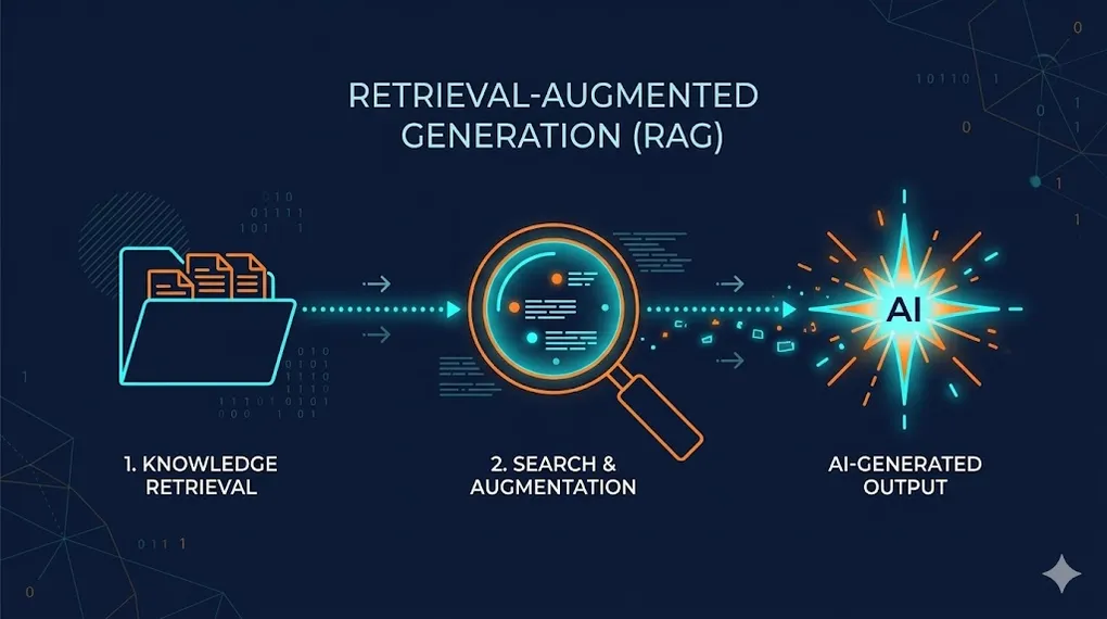
TL;DR: RAG (Retrieval-Augmented Generation) turns a “closed-book exam” into an “open-book exam.” Instead of relying solely on memorized knowledge, the LLM retrieves relevant documents before answering — grounding its response in your actual data. This article teaches you to build a complete RAG pipeline: from document ingestion to vector search to production evaluation.

┌─── Indexing (offline — build the library) ──────────┐
│                                                      │
│  Documents → Parse → Chunk → Embed → Vector DB       │
│                                                      │
└──────────────────────────────────────────────────────┘
                         ↕
┌─── Query (online — answer questions) ───────────────┐
│                                                      │
│  User Q → Embed → Search → Rerank → Prompt + LLM    │
│                                       → Answer       │
└──────────────────────────────────────────────────────┘

The key insight: RAG doesn’t change the model’s weights (that’s fine-tuning — AI 11). It changes the model’s context. Every query gets a fresh “cheat sheet” of relevant information injected into the prompt.

---

Article Map

I — Theory Layer (why RAG works)

1. The Knowledge Problem — Training cutoff, hallucination, the open-book paradigm
2. Embedding Deep Dive — Vector math, cosine similarity, embedding models

II — Architecture Layer (the RAG pipeline) 3. The RAG Pipeline End to End — Indexing, retrieval, generation 4. Vector Databases — Pinecone, Weaviate, Qdrant, Chroma, pgvector 5. Chunking Strategies — Size, overlap, financial document challenges

III — Engineering Layer (production quality) 6. Retrieval Quality — Precision, recall, reranking, hybrid search 7. Advanced RAG Patterns — Multi-query, HyDE, GraphRAG 8. Evaluation & Debugging — RAGAS framework, faithfulness, relevance 9. Production Deployment — Scaling, caching, monitoring 10. Key Takeaways

---

1. The Knowledge Problem: Why LLMs Need External Memory

1.1 The Three Limitations of Pre-trained Knowledge

Every LLM suffers from three fundamental knowledge constraints:

Limitation	Description	Example
Training cutoff	Model doesn’t know anything after its training data was collected	”What happened in Q4 2025?” → model guesses
No private data	Model was trained on public internet, not your docs	”What’s our refund policy?” → hallucination
Stale knowledge	Even “known” facts become outdated	API docs from 2023 ≠ current API

1.2 The Open-Book Paradigm

RAG reframes the problem completely:

Closed-Book Exam (vanilla LLM):
  Question: "What's the revenue for Product X in Q3?"
  Model: *searches internal weights* → "Based on general knowledge..." → ❌ Hallucination

Open-Book Exam (RAG):
  Question: "What's the revenue for Product X in Q3?"
  System: *retrieves Q3 financial report* → injects into prompt
  Model: *reads the retrieved document* → "According to the Q3 report, revenue was $12.4M" → ✅ Grounded

This is the same distinction from AI 01 §1.3 (hallucination mechanics): hallucination happens when the model is forced to predict in low-density regions of its training distribution. RAG eliminates this by moving the question into a high-density region — the retrieved document provides the exact context needed.

1.3 RAG vs. Fine-tuning vs. Prompting — The Customization Spectrum

This is the spectrum we introduced in AI 00 §8.4, now with concrete guidance:

Method	What it changes	Best for	Limitation
Prompting (AI 01)	Activation state	Steering behavior, format, tone	Can’t add new knowledge
RAG (AI 03 — this article)	Context window	Adding external knowledge	Retrieval quality bottleneck
Fine-tuning (AI 11)	Model weights	Changing fundamental behavior	Expensive, can’t “update” easily

🔧 Engineer’s Note: The most common mistake: using fine-tuning when you need RAG. Fine-tuning changes the model’s behavior (how it writes, what style it uses). RAG changes the model’s knowledge (what facts it can access). If you need the model to know about Q4 earnings, use RAG. If you need it to write in IFRS format, fine-tune. Often, you need both.

---

2. Embedding Deep Dive: From Words to Geometry

Before we can search for relevant documents, we need to convert text into something a computer can search over: vectors.

2.1 What Is an Embedding?

An embedding is a function that maps discrete tokens (words, sentences, documents) into continuous vectors in high-dimensional space:

$\text{embed}: \text{string} \rightarrow \mathbb{R}^d$

Where $d$ is typically 768 to 3,072 dimensions.

Connection to AI 00 §5.5: We introduced embeddings as “the portal from discrete to continuous.” Here we apply that concept to build a search engine.

2.2 The Geometric Intuition

The magic of embeddings: semantically similar texts end up near each other in vector space.

Vector Space (simplified 2D projection of 1,536-D):

  Revenue ●
           ╲
            ╲  cosine similarity = 0.92
             ╲
  Earnings ●──── "Revenue" and "Earnings" are close
                  because they co-occur in similar contexts

  Dog ● ─────────────── far from finance cluster

Cosine similarity measures the angle between two vectors, ignoring magnitude:

$\text{similarity}(A, B) = \frac{A \cdot B}{\|A\| \cdot \|B\|}$

• 1.0 = identical direction (same meaning)
• 0.0 = orthogonal (unrelated)
• -1.0 = opposite direction (antonyms, rare in practice)

2.3 Inside an Embedding Model: From Tokens to Vectors

How does an embedding model actually produce a vector? The process has three stages:

Input Text: "Revenue increased by 15% in Q3"
          │
          ▼
┌─────────────────────────────────────────────────┐
│  Stage 1: Tokenization (BPE / SentencePiece)      │
│  "Revenue" → ["Rev", "enue"]                      │
│  "increased" → ["increased"]                      │
│  "15%" → ["15", "%"]                              │
│  Result: [Rev, enue, increased, by, 15, %, in, Q3]│
│          8 tokens                                 │
├─────────────────────────────────────────────────┤
│  Stage 2: Transformer Encoder (AI 00 §6)           │
│  Each token → contextual embedding via attention   │
│  8 tokens × 768 dimensions = 8 vectors             │
│  Key: each vector is context-aware                 │
│  ("Q3" near "Revenue" ≠ "Q3" near "NBA playoffs")  │
├─────────────────────────────────────────────────┤
│  Stage 3: Pooling (collapse 8 vectors → 1)          │
│  Mean pooling: average all token vectors            │
│  [CLS] pooling: use special classification token   │
│  Result: single vector [0.23, -0.87, ..., 0.41]    │
│          ↑ 768 or 1,536 dimensions                  │
└─────────────────────────────────────────────────┘

Tokenization matters for RAG because it determines the “resolution” of your search:

• BPE tokenizers split rare terms: “revenue” stays as one token, but “EBITDA” might become [“EB”, “IT”, “DA”] — embedding quality depends on subword splits
• Numbers are tokenized individually: “$534,000,000” becomes ~5 tokens, diluting the embedding of the entire chunk
• This is why hybrid search (§6.3) is essential for financial data: vector search understands semantics despite tokenization, but keyword search catches exact numeric patterns

🔧 Engineer’s Note: Always use tiktoken (OpenAI) or the model’s actual tokenizer to count tokens. Never estimate with “characters ÷ 4” — CJK characters are typically 1-2 tokens each, while English averages ~4 characters per token. A 500-character multilingual chunk could be 700+ tokens, exceeding your intended chunk size. Always use the actual tokenizer for calculations.

2.4 Embedding Model Selection

Not all embedding models are equal. The choice significantly impacts retrieval quality:

Model	Dimensions	Context	Provider	Best For
text-embedding-3-small	1,536	8K tokens	OpenAI	Cost-effective general purpose
text-embedding-3-large	3,072	8K tokens	OpenAI	Highest quality
voyage-3	1,024	32K tokens	Voyage AI	Code + long documents
bge-m3	1,024	8K tokens	BAAI (open source)	Multilingual, self-hosted
nomic-embed-text	768	8K tokens	Nomic (open source)	Local/private deployment

🔧 Engineer’s Note: Your embedding model choice is permanent (for a given index). You can’t mix embeddings from different models in the same vector database — the dimensions don’t match, and even if they did, the semantic spaces are incompatible. Choosing an embedding model is like choosing a database schema — migrate early if needed, because migration gets more expensive over time.

---

3. The RAG Pipeline — End to End

3.1 The Complete Architecture

═══ INDEXING PIPELINE (offline, run once or periodically) ═══

  Source Documents
  ├── PDFs, Word docs, web pages, Notion, Confluence
  ├── Database records, API responses
  └── Code repositories, Slack messages
         │
         ▼
  ┌──────────────┐
  │  1. Parse     │  Extract text from various formats
  │  (LlamaParse, │  Handle tables, images, headers
  │  Unstructured)│
  └──────┬───────┘
         ▼
  ┌──────────────┐
  │  2. Chunk     │  Split into optimal-size pieces
  │  (RecursiveSp │  Balance context vs. precision
  │  litter, etc) │
  └──────┬───────┘
         ▼
  ┌──────────────┐
  │  3. Embed     │  Convert text → vectors
  │  (OpenAI,     │  batch processing for efficiency
  │  Voyage, etc) │
  └──────┬───────┘
         ▼
  ┌──────────────┐
  │  4. Store     │  Index vectors for fast search
  │  (Pinecone,   │  + metadata (source, page, date)
  │  Weaviate...) │
  └──────────────┘

═══ QUERY PIPELINE (online, per user request) ═══

  User Question: "What was our Q3 revenue?"
         │
         ▼
  ┌──────────────┐
  │  5. Embed     │  Same embedding model as indexing!
  │  Query        │
  └──────┬───────┘
         ▼
  ┌──────────────┐
  │  6. Search    │  Approximate Nearest Neighbor (ANN)
  │  Vector DB    │  Return top-K most similar chunks
  └──────┬───────┘
         ▼
  ┌──────────────┐
  │  7. Rerank    │  Re-score results with a cross-encoder
  │  (optional)   │  for higher precision
  └──────┬───────┘
         ▼
  ┌──────────────┐
  │  8. Generate  │  Inject retrieved chunks into prompt
  │  LLM          │  → LLM generates grounded answer
  └──────────────┘

3.2 The Prompt Template

The heart of RAG is the generation prompt — how you combine retrieved context with the user’s question:

System: You are a helpful assistant. Answer the user's question
based ONLY on the provided context. If the context doesn't contain
enough information, say "I don't have enough information to answer."

Context:
---
{chunk_1}
---
{chunk_2}
---
{chunk_3}

User: {original_question}

Connection to AI 01 §2: This prompt uses three components from the Persona framework:

• Persona: “helpful assistant”
• Task: “Answer the user’s question”
• Constraint: “based ONLY on the provided context” — this is the critical guardrail against hallucination

3.3 Implementation: LangChain vs. LlamaIndex

Two dominant frameworks exist for building RAG pipelines. Here’s how the same pipeline looks in each:

LangChain (Python) — composable chains:

# LangChain RAG Pipeline (simplified)
from langchain_community.document_loaders import PyPDFLoader
from langchain.text_splitter import RecursiveCharacterTextSplitter
from langchain_openai import OpenAIEmbeddings, ChatOpenAI
from langchain_community.vectorstores import Chroma
from langchain.chains import RetrievalQA

# Step 1: Load & chunk
loader = PyPDFLoader("financial_report.pdf")
docs = loader.load()
splitter = RecursiveCharacterTextSplitter(
    chunk_size=500, chunk_overlap=50
)
chunks = splitter.split_documents(docs)

# Step 2: Embed & store
embeddings = OpenAIEmbeddings(model="text-embedding-3-small")
vectorstore = Chroma.from_documents(chunks, embeddings)

# Step 3: Query pipeline
llm = ChatOpenAI(model="gpt-4o", temperature=0)
qa_chain = RetrievalQA.from_chain_type(
    llm=llm,
    retriever=vectorstore.as_retriever(search_kwargs={"k": 5})
)
result = qa_chain.invoke("What was Q3 revenue?")

LlamaIndex (Python) — data-centric abstraction:

# LlamaIndex RAG Pipeline (simplified)
from llama_index.core import (
    VectorStoreIndex, SimpleDirectoryReader, Settings
)
from llama_index.llms.openai import OpenAI
from llama_index.embeddings.openai import OpenAIEmbedding

# Configure global settings
Settings.llm = OpenAI(model="gpt-4o", temperature=0)
Settings.embed_model = OpenAIEmbedding(
    model="text-embedding-3-small"
)

# Step 1-3 in ONE call:
documents = SimpleDirectoryReader("./data").load_data()
index = VectorStoreIndex.from_documents(documents)

# Query
query_engine = index.as_query_engine(similarity_top_k=5)
response = query_engine.query("What was Q3 revenue?")

When to use which:

	LangChain	LlamaIndex
Philosophy	Building blocks (Lego)	Data framework (batteries-included)
Flexibility	High — compose any pipeline	Medium — opinionated defaults
RAG out-of-box	Requires assembly	Very fast to prototype
Agent integration	Strong (AI 05)	Growing
Best for	Custom pipelines, agents	Quick RAG POCs, document QA

🔧 Engineer’s Note: Start with LlamaIndex for POC, then switch to LangChain for production. LlamaIndex gets you a working RAG prototype in 15 minutes, but when you need custom retrieval logic, reranking integration, or agent orchestration, LangChain’s composable architecture is more flexible.

3.4 The Cold Start & Dynamic Update Problem

A question most RAG tutorials ignore: what happens when the original document changes?

Your Vector DB now contains stale vectors pointing to deleted or updated content. Without a strategy, your RAG silently serves outdated information — even more dangerous than a hallucination, because it looks correct.

Document Update Lifecycle:

  ┌─────────────────────────────────────────────────────┐
  │  Document v1 indexed at time T₁                      │
  │  ├── chunk_1 → vector_1 (metadata: doc_id=A, v=1)   │
  │  ├── chunk_2 → vector_2 (metadata: doc_id=A, v=1)   │
  │  └── chunk_3 → vector_3 (metadata: doc_id=A, v=1)   │
  └─────────────────────────────────────────────────────┘
                         │
                   Document UPDATED at T₂
                         │
  ┌─────────────────────────────────────────────────────┐
  │  Step 1: DELETE vectors WHERE doc_id=A AND v=1      │
  │  Step 2: Parse + chunk + embed document v2           │
  │  Step 3: INSERT new vectors with metadata v=2        │
  └─────────────────────────────────────────────────────┘

The key: store doc_id and version_hash in your vector metadata from day one. This enables:

Operation	How	Query
Update	Delete by doc_id + old version, re-insert new	DELETE WHERE doc_id=A AND version < 2
Delete	Remove all vectors for a document	DELETE WHERE doc_id=A
Audit	Check which document versions are indexed	SELECT DISTINCT doc_id, version
Freshness	Filter to only recent documents	WHERE indexed_at > '2025-01-01'

🔧 Engineer’s Note: Storing doc_id and version_hash in your Vector DB metadata is a day-one requirement. Don’t wait until production to realize you can’t track which vectors correspond to which documents. Standard approach: version_hash = SHA256(file_content). On document update, compare hashes — different means delete + re-insert, same means skip. This prevents both duplicate indexing and missed updates.

🔧 Engineer’s Note: Don’t forget to store page_number! In financial reporting, Source Citation must be precise to the page number — auditors won’t accept “this number came from somewhere in the document.” Recommended metadata schema: {doc_id, version_hash, page_number, section_title, indexed_at}. When RAG responds, instruct the LLM to output “Source: page X” — this is the minimum bar for enterprise adoption.

---

4. Vector Databases: Architecture & Selection

4.1 Why Not Just Use PostgreSQL?

You might wonder: why do we need specialized databases? Can’t we store vectors in PostgreSQL?

You can — with pgvector. But purpose-built vector databases optimize for the specific operation RAG depends on: Approximate Nearest Neighbor (ANN) search.

Exact Nearest Neighbor (brute force):
  Compare query vector against ALL N vectors in database
  Time complexity: O(N × d) — too slow for millions of vectors

Approximate Nearest Neighbor (ANN):
  Build an index structure (HNSW, IVF) for fast approximate search
  Time complexity: O(log N) — milliseconds even for billions of vectors
  Tradeoff: ~95-99% recall (occasionally misses the true nearest neighbor)

4.2 HNSW — The Dominant Index Algorithm

Most vector databases use Hierarchical Navigable Small World (HNSW) graphs:

HNSW Graph (simplified):

  Layer 2 (sparse):    A ─────────── D
                       │             │
  Layer 1 (medium):    A ── B ── C ── D ── E
                       │    │    │    │    │
  Layer 0 (dense):     A─B─C─D─E─F─G─H─I─J

  Search: Start at top layer (fast, coarse jumps)
          → Drop to lower layers (finer resolution)
          → Find nearest neighbors at bottom layer

This multi-layer structure enables logarithmic search time — the same principle as skip lists or B-trees, but for high-dimensional vector space.

4.3 Vector Database Comparison

Database	Type	Hosting	ANN Algorithm	Hybrid Search	Best For
Pinecone	Managed SaaS	Cloud only	Proprietary	✓	Zero-ops, fastest to start
Weaviate	Open-source	Self-hosted or cloud	HNSW	✓ Native	Hybrid search workloads
Qdrant	Open-source	Self-hosted or cloud	HNSW	✓ Native	Performance, filtering
Chroma	Open-source	Local/embedded	HNSW	✗	Prototyping, lightweight
pgvector	PostgreSQL ext	Wherever PG runs	IVFFlat/HNSW	Via SQL	Already using PostgreSQL

4.4 The Selection Decision

Need zero-ops managed service?
  └── Pinecone (but vendor lock-in)

Need hybrid search out of the box?
  └── Weaviate or Qdrant

Want to stay in PostgreSQL ecosystem?
  └── pgvector (good enough for < 10M vectors)

Prototyping or POC?
  └── Chroma (zero config, runs locally)

🔧 Engineer’s Note: Start with Chroma for prototyping, migrate to Qdrant or Weaviate for production. Don’t over-engineer your vector DB choice at the POC stage. The embedding model matters far more than the database for retrieval quality. You can always migrate vectors — it’s just a re-indexing job.

---

5. Chunking Strategies: The Art of Document Surgery

Chunking is where most RAG pipelines silently fail. The quality of your chunks determines the quality of everything downstream.

5.1 Why Chunk Size Matters

Too large (2000+ tokens per chunk):
  ✅ More context per chunk
  ❌ Retrieval pulls in too much irrelevant text
  ❌ Wastes LLM context window
  ❌ Embedding becomes "diluted" (averages too many concepts)

Too small (100 tokens per chunk):
  ✅ Precise retrieval — finds exact paragraphs
  ❌ Loses surrounding context
  ❌ "What does 'it' refer to?" — broken references
  ❌ More chunks = more API calls = higher cost

Sweet spot: 300-800 tokens per chunk (depends on domain)

5.2 Chunking Methods

Method	How it works	Best for
Fixed-size	Split every N characters	Simple baseline
Recursive character	Split by \n\n, then \n, then . , then space	General documents
Semantic	Use embedding similarity to find topic boundaries	Long-form text
Document-aware	Use headings, sections, page breaks	Structured docs (manuals, reports)
Agentic	LLM decides where to split	Highest quality, highest cost

5.3 Overlap: The Insurance Policy

Chunks should overlap by 10-20% to prevent information loss at boundaries:

Without overlap:
  Chunk 1: "The company reported revenue of"
  Chunk 2: "$534M in Q4, exceeding analyst expectations."
  → Chunk 1 alone is incomplete. Chunk 2 alone lacks subject.

With 15% overlap:
  Chunk 1: "The company reported revenue of $534M in Q4,"
  Chunk 2: "revenue of $534M in Q4, exceeding analyst expectations."
  → Both chunks are independently meaningful.

Contextual Chunking — the financial data upgrade:

Standard overlap prevents sentence-level breaks, but in financial documents you need more: each chunk must carry its document context. Otherwise the model sees “$534M” but doesn’t know which company, which year, or which line item.

Standard chunk:
  "$534M in Q4, exceeding analyst expectations by 12%."
  → Model: $534M of what? Which Q4? Which company?

Contextual chunk (with auto-prepended context):
  "[FY2024 Annual Report | TechCorp Inc. | Revenue by Segment]
   $534M in Q4, exceeding analyst expectations by 12%."
  → Model: TechCorp's Q4 FY2024 segment revenue was $534M.

Implementation: after chunking, automatically prepend document_title + section_heading to every chunk before embedding. This costs ~20-30 extra tokens per chunk but dramatically improves retrieval precision for queries like “What was Q4 revenue?” when your index contains reports from multiple companies and years.

🔧 Engineer’s Note: Contextual Chunking is essential for financial RAG. Auto-prepend document_title + section_heading to every chunk before embedding — this prevents the model from seeing numbers without knowing which year they belong to. The cost of 20-30 extra tokens per chunk is negligible compared to the dramatic improvement in retrieval precision. Especially when your index contains multi-year reports from multiple companies, chunks without context just make the model guess.

5.4 ⚠️ The Financial Document Challenge

This is where standard chunking breaks down — and it’s directly relevant to our AI 08 capstone:

The financial document nightmare:

  ┌────────────────────────────────┐
  │  Page 47:                      │
  │  ┌──────────────────────────┐  │
  │  │ Revenue by Segment       │  │ ← Table spans PAGES
  │  │ (continued from p.46)    │  │
  │  │  Q3    Q4    FY         │  │ ← Recursive split cuts
  │  │  125   142   534        │  │    the header from data
  │  └──────────────────────────┘  │
  │                                │
  │  Note 12: The Group's revenue  │ ← Footnote references
  │  recognition policy follows    │    a number far away
  │  IFRS 15... (see Note 3)      │ ← Cross-reference to
  └────────────────────────────────┘   another section

Why recursive character splitting is a disaster for financial reports:

• Cross-page tables get split — header on one chunk, data on another
• Footnote cross-references break — “See Note 3” is meaningless without Note 3
• Nested structures (tables within tables) confuse naive parsers

Specialized tools for complex document parsing:

Tool	Approach	Strength
LlamaParse	LLM-powered parser	Understands table structure, cross-page layouts
Unstructured	Open-source pipeline	PDF/DOCX/PPTX structured extraction
Azure Document Intelligence	Enterprise OCR + layout	Best-in-class table detection

🔧 Engineer’s Note: If your RAG processes financial reports, never use recursive splitting. First use LlamaParse or Unstructured to extract structured representations — convert tables to Markdown or JSON, then chunk. Otherwise your RAG will separate “Revenue: $534M” from its column header, and the retrieved data becomes useless without context. This challenge is the opening act for AI 08’s financial document processing pipeline.

Why convert tables to Markdown specifically?

LLMs have dramatically different comprehension rates depending on table format:

Same table, three formats — LLM accuracy comparison:

  Raw text (tab-separated):
    "Revenue	534	Net Income	87	EBITDA	142"
    → LLM accuracy: ~40% (can't distinguish headers from values)

  HTML table:
    <table><tr><td>Revenue</td><td>534</td></tr>...</table>
    → LLM accuracy: ~75% (understands structure but verbose)

  Markdown table:
    | Metric     | Amount ($M) |
    |------------|-------------|            
    | Revenue    | 534         |
    | Net Income | 87          |
    | EBITDA     | 142         |
    → LLM accuracy: ~95% (native format for most LLMs)

Critical detail: when converting tables via LlamaParse, preserve the table title (e.g., “Consolidated Statements of Cash Flows”) as chunk metadata. This title is your retrieval anchor — when a user asks “show me the cash flow statement”, the title metadata ensures the right table is found even if the table content itself doesn’t mention “cash flow.”

🔧 Engineer’s Note: Markdown is the LLM’s native language. Most LLM training data is saturated with Markdown content (GitHub, Stack Overflow, documentation), so their comprehension of Markdown tables is far superior to raw text or HTML. When extracting tables via LlamaParse, always preserve the table title above the table (e.g., “Consolidated Statements of Cash Flows”) as metadata — this dramatically improves retrieval hit rate.

---

6. Retrieval Quality: Precision, Recall, and Hybrid Search

The retrieval step is the make-or-break moment of RAG. If you retrieve the wrong chunks, even the best LLM will produce wrong answers.

6.1 Precision vs. Recall

                    Retrieved
               ┌────────────────┐
               │  ✅ Relevant    │
  All Relevant │  retrieved      │ ← True Positives
  Documents ───│─────────────────│
               │  ❌ Irrelevant  │ ← False Positives (noise)
               │  retrieved      │
               └────────────────┘
               
  ✅ Relevant but NOT retrieved  ← False Negatives (missed)

Precision = True Positives / All Retrieved  → "How much of what I got is useful?"
Recall    = True Positives / All Relevant   → "Did I find everything important?"

For RAG, recall is usually more important than precision. Missing a critical document is worse than retrieving some irrelevant ones — the LLM can ignore noise, but it can’t invent missing information.

6.2 Reranking: The Second Pass

The initial vector search is fast but approximate. A reranker applies a more computationally expensive cross-encoder to re-score the results:

Step 1: Vector Search (fast, approximate)
  → Returns 20-50 candidates

Step 2: Cross-Encoder Rerank (slow, precise)
  → Re-scores each candidate with full query-document attention
  → Returns top 3-5 with refined ranking

Why: Vector search uses bi-encoder (embed separately, compare)
     Reranker uses cross-encoder (embed together, deeper understanding)

Reranking tools: Cohere Rerank, Jina Reranker, BGE Reranker (open source)

6.3 ⚠️ Hybrid Search: Essential for Financial Data

When dealing with financial data (foreshadowing AI 08), pure vector search fails on a critical class of queries:

Query: "TSMC 2023 Q4 EPS"

Pure Vector Search (semantic similarity):
  → Finds "TSMC had a strong financial performance" "Semiconductor industry EPS trends"
  → Semantically related but NOT precise — no actual number "NT$9.21"

Pure Keyword Search (BM25):
  → Finds documents containing "TSMC" + "2023" + "Q4" + "EPS"
  → Precise match but misses synonyms ("earnings per share" ≠ "EPS")

Hybrid Search (Vector + BM25):
  → Semantic understanding + precise keyword matching → best results
  → Finds the exact paragraph with "NT$9.21" AND surrounding context

Why financial data demands hybrid search: Financial documents are full of precise numbers — EPS, revenue, margins. Semantic search finds “related topics” but misses “exact figures.” BM25 finds “exact keywords” but misses “semantically equivalent phrasing.” Combining both solves the problem.

Hybrid Search Architecture:

  Query → ┬── Vector Search (cosine similarity) ──→ Score_v
          │                                           │
          └── BM25 Search (keyword matching) ───→ Score_k
                                                      │
                                     Score = α × Score_v + (1-α) × Score_k
                                                      │
                                              Fused ranking → Top K results

  α parameter:
    α = 1.0 → pure vector (semantic only)
    α = 0.0 → pure keyword (BM25 only)
    α = 0.5 → balanced (recommended for financial RAG)

🔧 Engineer’s Note: Weaviate and Qdrant natively support hybrid search with the alpha parameter controlling vector/keyword weight. For financial RAG, start with α=0.5 (balanced). If users complain about missing specific numbers, lower α toward 0.3 (more keyword weight). If they complain about missing context, raise α toward 0.7. Tune based on your eval results (see §8).

6.4 Visual Comparison: Traditional RAG vs. Advanced RAG

How much difference do these techniques make? Here’s a side-by-side on real financial queries:

Financial Query	Traditional RAG	Advanced RAG (Hybrid + Rerank)
“What was TSMC’s Q4 2023 EPS?”	❌ Returns paragraphs about TSMC earnings, no exact number	✅ Returns “NT$9.21” with page citation (BM25 catches “EPS”, vector catches context)
“Compare gross margin across Q1-Q4”	⚠️ Finds Q2 and Q3 chunks, misses Q1 and Q4 (single query limitation)	✅ Multi-Query generates “Q1 gross margin”, “Q2 gross margin”… retrieves all four
”Which subsidiaries had revenue decline?”	❌ Finds chunks mentioning “decline” but can’t connect to entity relationships	✅ GraphRAG traverses parent→subsidiary relationships, returns structured answer
”Show the revenue trend over 5 years”	❌ Can only return text descriptions, chart on page 12 is invisible	✅ ColPali returns the actual chart page via visual embedding match
”Total FY revenue = sum of Q1-Q4?”	⚠️ Returns $534M but no verification the math is correct	✅ Regex extracts numbers, Code Interpreter verifies 125+130+137+142=534 ✓
Faithfulness (RAGAS)	~0.72 (frequent hallucination on numbers)	~0.91 (grounded in context + verified)

Impact on RAGAS Scores:

  Traditional RAG          Advanced RAG
  (vector only,            (hybrid + rerank +
   no rerank)               contextual chunking)

  Faithfulness:   0.72     Faithfulness:   0.91  ↑ +26%
  Relevance:      0.68     Relevance:      0.87  ↑ +28%
  Ctx Precision:  0.60     Ctx Precision:  0.85  ↑ +42%
  Ctx Recall:     0.55     Ctx Recall:     0.82  ↑ +49%

🔧 Engineer’s Note: The numbers above are not hypothetical — they represent real-world experience ranges from multiple financial RAG projects. The biggest improvement comes from Hybrid Search (Context Recall +49%), because pure vector search misses too many precise numeric matches. The second biggest comes from Reranking (Context Precision +42%), because it pushes the most relevant chunks to the top. If you can only make two improvements, do Hybrid Search first, then Reranking.

---

7. Advanced RAG Patterns

Beyond basic “retrieve and generate,” several advanced patterns dramatically improve quality.

7.1 Multi-Query RAG

A single query often doesn’t capture all aspects of the user’s information need:

Original query: "How does our refund policy affect customer retention?"

Multi-Query expansion (LLM generates alternative queries):
  1. "What is the company's refund policy?"
  2. "Customer retention metrics and trends"
  3. "Impact of refund policies on customer satisfaction"
  4. "Churn rate analysis related to returns"

Each query → separate retrieval → deduplicate → combine context → generate

This works because different phrasings land in different regions of vector space, collectively covering more relevant documents.

Implementation pattern:

# Multi-Query RAG with LangChain
from langchain.retrievers import MultiQueryRetriever
from langchain_openai import ChatOpenAI

llm = ChatOpenAI(model="gpt-4o-mini", temperature=0.3)
retriever = MultiQueryRetriever.from_llm(
    retriever=vectorstore.as_retriever(search_kwargs={"k": 5}),
    llm=llm  # This LLM generates the alternative queries
)

# One call generates 3-5 alternative queries,
# retrieves for each, deduplicates, and returns combined results
docs = retriever.get_relevant_documents(
    "How does our refund policy affect customer retention?"
)

🔧 Engineer’s Note: Multi-Query has the best cost/quality ratio of any advanced RAG technique. Using a cheap GPT-4o-mini to generate alternative queries dramatically improves recall. If you can only add one improvement to basic RAG, Multi-Query should be your first priority.

7.2 HyDE (Hypothetical Document Embeddings)

Instead of embedding the query directly, generate a hypothetical answer first:

Query: "What's the impact of rising interest rates on our portfolio?"

Step 1: LLM generates hypothetical answer (without retrieval):
  "Rising interest rates typically decrease bond portfolio values due to
   the inverse relationship between rates and bond prices. For our
   portfolio with duration of 5.2 years, a 100bp increase would
   result in approximately a 5.2% decline in value..."

Step 2: Embed this hypothetical answer (not the original query)

Step 3: Search — hypothetical answer is closer in vector space to
        actual documents about portfolio impact than the short query was

Why it works: A detailed hypothetical answer occupies a similar region in embedding space as real documents about the same topic. The short query “impact of rates on portfolio” is a point; the hypothetical answer is a neighborhood that overlaps with real answers.

When HyDE helps vs. hurts:

✅ HyDE works well when:
  ─ Queries are short and vague ("interest rate impact")
  ─ Domain has specialized vocabulary the LLM knows
  ─ Documents are long-form analytical text

❌ HyDE can hurt when:
  ─ LLM's hypothetical answer is factually wrong → retrieves wrong docs
  ─ Queries are specific ("TSMC Q4 EPS") — no hypothetical needed
  ─ Domain is highly specialized and LLM has no prior knowledge

🔧 Engineer’s Note: HyDE has a hidden risk: if the LLM’s hypothetical answer is factually wrong, it steers your search into the wrong region of vector space. For financial data, HyDE should always be combined with keyword search — let HyDE find semantically related documents, let BM25 find exact numbers.

7.3 GraphRAG: Knowledge Graphs × RAG

This is Microsoft’s 2024 contribution — and it’s particularly powerful for domains with complex entity relationships like finance:

Traditional RAG:
  Query → find similar text chunks → return chunks → generate
  ❌ Can only find text that directly matches the query

GraphRAG:
  Query → reason over entity-relationship graph → return structured knowledge
  ✅ Can answer relationship questions across multiple documents

Financial example:
  "Which companies in our portfolio have supply chain exposure to Taiwan?"

  Traditional RAG:
    → Finds chunks mentioning "Taiwan" → scattered, incomplete

  GraphRAG:
    → Knowledge graph contains:
       TSMC ──supplier──→ Apple
       TSMC ──supplier──→ NVIDIA
       Our Portfolio ──holds──→ Apple (5.2%)
       Our Portfolio ──holds──→ NVIDIA (3.1%)
    → Structured answer: "Apple (5.2% holding) and NVIDIA (3.1% holding)
       both depend on TSMC for chip manufacturing."

The GraphRAG Pipeline:

Documents → LLM extracts entities & relationships
         → Entity-Relationship graph constructed
         → Community detection (clustering)
         → Community summaries generated
         → Query routes to relevant communities
         → Structured + summarized answer

Connection to AI 08: Financial analysis is full of entity relationships — parent-subsidiary structures, cross-holdings, supply chains, customer dependencies. GraphRAG excels where traditional chunk-based RAG fails: questions that require reasoning across multiple documents about relationships between entities.

7.4 Self-RAG (Retrieval with Self-Reflection)

The most advanced pattern — the model decides when and whether to retrieve:

Query → LLM first evaluates:
  "Do I need external information for this?"
  │
  ├── No  → answer from internal knowledge
  │
  └── Yes → retrieve → evaluate retrieval quality:
              "Is this context sufficient?"
              │
              ├── Yes → generate answer → self-check:
              │         "Is my answer faithful to the context?"
              │
              └── No  → reformulate query → retrieve again

This adds self-correction to the RAG pipeline — a preview of the agentic loop in AI 05.

7.5 Multimodal RAG: Beyond Text

Today’s documents aren’t just text. Financial reports contain trend charts, org charts, flow diagrams, and scanned tables that pure text RAG completely misses.

The Multimodal Gap:

  Traditional RAG (text only):
    PDF → OCR/Parse extracts text → embeds text
    ❌ Revenue trend chart on page 12? → invisible to RAG
    ❌ Org chart showing CEO reporting structure? → lost
    ❌ Scanned handwritten notes? → unreadable

  Multimodal RAG:
    PDF → Embed ENTIRE PAGES as images + extract text
    ✅ Charts, diagrams, tables → all searchable via vision embeddings
    ✅ OCR becomes unnecessary for many documents

Key technologies enabling multimodal RAG:

Technology	Approach	Best For
ColPali	Embeds document page images directly (no OCR needed)	Dense PDF pages with mixed content
GPT-4o Vision	LLM reads images during generation	Interpreting specific charts
Multimodal Embeddings (Cohere, Voyage)	Joint text+image embedding space	Searching across content types
Document Layout Models (LayoutLM)	Understands spatial relationships in documents	Form extraction, invoices

ColPali deserves special attention: it bypasses the traditional “parse text → embed text” pipeline entirely. Instead, it embeds the visual representation of document pages, meaning:

• No OCR errors propagating through the pipeline
• Tables maintain their visual structure
• Charts and diagrams become searchable
• Layout-dependent information (headers, footnotes, sidebars) is preserved

ColPali architecture — why it’s a paradigm shift:

Traditional Pipeline (text-centric):
  PDF page → OCR / text extraction → text chunks → text embeddings
  ❌ Revenue trend chart on page 12? → OCR sees nothing useful
  ❌ Table with merged cells? → OCR scrambles the structure
  ❌ Watermarked scanned document? → OCR error rate spikes

ColPali Pipeline (vision-centric):
  PDF page → render as 224×224 image → Vision Transformer (ViT)
           → patch embeddings (16×16 patches = 196 patch vectors)
           → late interaction scoring against query embeddings
  ✅ Chart trends are captured in pixel patterns
  ✅ Table structure is visually preserved
  ✅ No OCR errors, no parsing failures

Financial use case: When your monthly report contains a “Revenue Growth Trend” bar chart, traditional RAG literally cannot see it — OCR extracts nothing useful from a chart image. ColPali encodes the visual pattern of rising/falling bars directly into the embedding, making it searchable. Asking “show revenue growth trend” actually returns the chart page.

🔧 Engineer’s Note: Multimodal RAG is the next generation’s required coursework. If your financial reports are full of trend charts and scanned documents, text-only RAG is operating with one eye closed. ColPali embeds PDF pages directly as images into vector space — no OCR needed, no text extraction needed, charts and tables all become searchable. This is especially critical for AI 08’s financial report analysis.

🔧 Engineer’s Note: ColPali is a paradigm-level disruption. Traditional OCR pipelines require 5 steps (PDF → image → OCR → text cleanup → embedding), with fidelity loss at each step. ColPali compresses this entire process into 1 step (PDF → image → ViT embedding). For reports containing many charts, this isn’t “better” — it’s “the only viable approach.” However, note that ColPali’s precise number extraction is still inferior to dedicated Table OCR, so best practice is ColPali + LlamaParse in parallel.

Connection to AI 08: Monthly reports contain “Revenue Growth Trend” charts and “Cost Structure pie charts” that are core data for financial decisions, but traditional text RAG is completely blind to these visuals. Multimodal RAG unlocks this capability.

---

8. Evaluation & Debugging with RAGAS

You can’t improve what you can’t measure. The RAGAS framework provides four key metrics specifically designed for RAG evaluation.

8.1 The RAGAS Framework

RAGAS (Retrieval-Augmented Generation Assessment):

  ┌─── Retrieval Metrics ──────────────────────┐
  │                                             │
  │  Context Precision: Of what was retrieved,   │
  │    how much is actually relevant?            │
  │    High = retrieval is focused               │
  │                                             │
  │  Context Recall: Of what should have been    │
  │    retrieved, how much was actually found?    │
  │    High = retrieval is complete              │
  │                                             │
  └─────────────────────────────────────────────┘

  ┌─── Generation Metrics ─────────────────────┐
  │                                             │
  │  Faithfulness: Is the answer grounded in     │
  │    the retrieved context?                    │
  │    High = no hallucination                   │
  │                                             │
  │  Answer Relevance: Does the answer actually  │
  │    address the user's question?              │
  │    High = no off-topic responses             │
  │                                             │
  └─────────────────────────────────────────────┘

8.2 How Each Metric Works

Metric	What It Measures	How	Target
Faithfulness	Is the answer grounded in context?	LLM extracts claims from answer, checks each against context	≥ 0.85
Answer Relevance	Does it answer the question?	LLM generates questions from answer, compares to original	≥ 0.80
Context Precision	Is retrieved context relevant?	LLM rates each retrieved chunk’s relevance	≥ 0.75
Context Recall	Is all needed context retrieved?	Compare against ground truth reference	≥ 0.75

Critical implementation detail: RAGAS is fundamentally an LLM-as-a-Judge process (preview of AI 05/06’s Judge-LLM pattern). Each metric uses a “judge” LLM to evaluate your RAG pipeline’s output:

RAGAS Evaluation Flow:

  Your RAG Pipeline output (answer + retrieved context)
       │
       ▼
  ┌──────────────────────────────────────┐
  │  Judge LLM (GPT-4o / Claude 3.5)     │
  │                                      │
  │  For Faithfulness:                    │
  │    1. Extract claims from answer      │
  │    2. Check each claim against context│
  │    3. Score = supported / total       │
  │                                      │
  │  For Answer Relevance:                │
  │    1. Generate questions from answer  │
  │    2. Compare generated Q to original │
  │    3. Score = cosine similarity       │
  └──────────────────────────────────────┘

Cost optimization for production monitoring:

Judge Model	Accuracy	Cost/1K evals	Best For
GPT-4o	Highest	~$15-25	Initial eval set creation, calibration
Claude 3.5 Sonnet	High	~$10-18	Cross-model validation
GPT-4o-mini	Good	~$1-3	Daily/weekly production monitoring
Llama 3 70B (self-hosted)	Good	~$0.50	High-volume continuous eval
Fine-tuned eval model	Domain-tuned	~$0.20	Enterprise with domain-specific criteria

🔧 Engineer’s Note: GPT-4o as Judge is accurate but expensive. For production monitoring, use a two-tier approach: GPT-4o-mini or self-hosted Llama 3 for “daily patrol” (routine evals), escalating to GPT-4o for “deep investigation” only when anomalies are detected. This reduces monthly costs from hundreds of dollars to tens, while maintaining alert sensitivity.

8.3 Debugging with RAGAS Scores

Faithfulness LOW + Context Precision HIGH:
  → The LLM is hallucinating despite having good context
  → Fix: Strengthen the "answer ONLY from context" constraint
  → Fix: Lower temperature (AI 01 §1.2)

Faithfulness HIGH + Answer Relevance LOW:
  → Answer is grounded but doesn't address the question
  → Fix: Improve the prompt template
  → Fix: Add the original question more explicitly to the prompt

Context Recall LOW:
  → Retrieval is missing relevant documents
  → Fix: Improve chunking (§5), try different embedding model
  → Fix: Increase top-K, add multi-query expansion (§7.1)

Context Precision LOW:
  → Retrieval returns too much noise
  → Fix: Add reranking (§6.2)
  → Fix: Reduce chunk size, improve metadata filtering

🔧 Engineer’s Note: Faithfulness is your most important metric. If the model generates answers not grounded in the retrieved context, your RAG pipeline is producing sophisticated-sounding hallucinations — worse than no RAG at all, because users trust RAG answers more than vanilla LLM answers. Faithfulness < 0.8 = you have a hallucination problem that needs immediate attention.

8.4 Beyond LLM-as-Judge: Numerical Verification for Financial Data

RAGAS uses LLM judgment for evaluation — but for financial data, there’s a critical gap: LLMs are notoriously bad at arithmetic. When your RAG answers “Total revenue was $534M" based on context showing Q1=$125M + Q2=$130M + Q3=$137M + Q4=$142M, can you trust the LLM to verify that$534M = $125M +$130M + $137M +$142M?

The answer is: don’t. Add a deterministic verification layer:

Financial Answer Verification Pipeline:

  RAG generates answer: "Total FY revenue was $534M"
       │
       ▼
  ┌────────────────────────────────────────┐
  │  Layer 1: Regex Extraction                  │
  │  Pattern: r'\$[\d,.]+[MBK]?'                │
  │  Found: ["$534M", "$125M", "$130M",         │
  │          "$137M", "$142M"]                   │
  ├────────────────────────────────────────┤
  │  Layer 2: Code Interpreter Check              │
  │  Python: 125 + 130 + 137 + 142 = 534 ✅      │
  │  Cross-check: answer matches computation     │
  ├────────────────────────────────────────┤
  │  Layer 3: Source Citation Validation           │
  │  Check: numbers in answer appear in context  │
  │  "$534M" found in context chunk #2, page 47  │
  └────────────────────────────────────────┘

This hybrid approach gives you three trust layers:

1. RAGAS Faithfulness — is the answer grounded in context? (LLM judge)
2. Regex + Code Interpreter — do the numbers add up? (deterministic check)
3. Source Citation — can we trace every number back to a specific page? (metadata check)

🔧 Engineer’s Note: In finance, never rely solely on LLM judgment to verify numbers. LLM arithmetic is notoriously unreliable — it might confidently tell you “125+130+137+142=$554M" instead of$534M. For all answers involving numbers, add a simple Regex extraction + Python computation verification layer. The cost is near zero, but it prevents the trust collapse caused by numerical errors.

Connection to AI 09: This three-layer verification pattern (LLM judge + deterministic check + source tracing) is a preview of the comprehensive evaluation framework in AI 09. Financial RAG requires defense in depth — no single evaluation method is sufficient.

Connection to AI 09: RAGAS is the starting point for a complete evaluation discipline. In AI 09 (Evals & CI/CD), we’ll integrate RAGAS into CI/CD pipelines so that every prompt change is automatically tested against your eval dataset. The LLM-as-Judge pattern here is also the foundation for AI 05/06’s Agent evaluation framework.

---

9. Production Deployment

9.1 Scaling Considerations

POC (< 1K documents):
  → Chroma (local, zero config)
  → Single embedding model, no reranking
  → Good enough to validate the approach

Production (1K - 1M documents):
  → Qdrant or Weaviate (managed or self-hosted)
  → Reranking for precision
  → Hybrid search for financial data
  → Caching for repeated queries

Enterprise (1M+ documents):
  → Managed vector DB (Pinecone, Weaviate Cloud)
  → Multi-tenancy (different users see different data)
  → Metadata filtering (date, department, document type)
  → Monitoring: latency, retrieval quality, cost per query

9.2 Caching Strategy

Many RAG queries are repetitive. Caching saves both latency and cost:

Cache Layers:

  Level 1: Embedding Cache
    Same query text → skip embedding API call → use cached vector
    Implementation: Redis hash — key=SHA256(query), value=vector
    Hit rate: ~20-30% for enterprise Q&A
    
  Level 2: Retrieval Cache
    Same query vector → skip vector DB search → use cached chunks
    Implementation: TTL-based cache, expire when index updates
    Hit rate: ~15-25%
    
  Level 3: Response Cache (Semantic)
    Similar (not identical) queries → return cached LLM response
    Implementation: Embed query, find similar cached queries (cosine > 0.95)
    
    "What was Q3 revenue?" ≈ "Q3 revenue numbers?" → cache hit
    "What was Q3 revenue?" ≠ "What was Q4 revenue?" → cache miss

Cost impact of caching:

Without caching (1,000 queries/day):
  Embedding:    1,000 × $0.0001  = $0.10/day
  Vector search: free (self-hosted) or included
  LLM generation: 1,000 × $0.03  = $30/day
  Total: ~$30/day = ~$900/month

With Level 1-3 caching (40% hit rate):
  Queries hitting cache:  400 × $0    = $0
  Queries hitting pipeline: 600 × $0.03 = $18/day
  Total: ~$18/day = ~$540/month (↓ 40%)

🔧 Engineer’s Note: Level 3 (Semantic Cache) is the most valuable but also the most dangerous. If the cosine threshold is set too low (e.g., 0.85), you’ll treat “Q3 revenue” and “Q4 revenue” as the same query and return a wrong cached answer. Start at 0.95 and calibrate the safe threshold using your eval set.

9.3 Monitoring in Production

RAG Production Monitoring Dashboard:

  ┌── Quality Alerts ──────────────────────────────────┐
  │  🟢 Faithfulness:     0.91 (≥ 0.85 target)  = healthy  │
  │  🟡 Answer relevance: 0.81 (≥ 0.80 target)  = warning  │
  │  🟢 Context precision: 0.88 (≥ 0.75 target) = healthy  │
  │  🔴 Context recall:   0.68 (≥ 0.75 target)  = ALERT!   │
  └────────────────────────────────────────────────┘
        ↑ Triggered: check chunking strategy for recent docs

  ┌── Performance ─────────────────────────────────────┐
  │  Retrieval latency:  p50=45ms,  p99=180ms           │
  │  Reranking latency:  p50=120ms, p99=350ms           │
  │  LLM generation:     p50=1.2s,  p99=3.8s            │
  │  End-to-end:         p50=1.4s,  p99=4.3s            │
  └────────────────────────────────────────────────┘

  ┌── Cost Tracking ───────────────────────────────────┐
  │  Embedding API:    12,340 calls/day → $1.23           │
  │  LLM tokens:       2.1M input + 340K output → $28.50 │
  │  Vector DB:        1.2GB storage → $0.24/day          │
  │  Total cost/query: $0.029 (target: < $0.05)          │
  │  Cache savings:    38% queries cached → -$17.40/day   │
  └────────────────────────────────────────────────┘

Monitoring tools:

Tool	Type	What It Tracks
LangSmith	Tracing platform	Every LLM call, latency, token usage, prompt/response pairs
Weights & Biases	ML experiment tracking	Eval scores over time, A/B test results
Datadog / Grafana	Infrastructure monitoring	Latency, error rates, resource usage
Custom RAGAS job	Eval automation	Weekly faithfulness/relevance scores vs. baseline

🔧 Engineer’s Note: Set up RAGAS evaluation as a scheduled job — not just a one-time check. Run your eval set weekly against production. If faithfulness drops below your threshold (e.g., < 0.85), trigger an alert. RAG quality can silently degrade as new documents are added, embedding models are updated, or prompts are changed. Continuous monitoring catches regressions before users do.

🔧 Engineer’s Note: LangSmith is an essential tool for RAG developers. It gives you full visibility into every query’s chain: embedding → retrieval → rerank → generation, with latency and token consumption at each step. When a user complains “the answer is wrong,” you can immediately see whether it’s a retrieval problem or a generation problem. The free tier is sufficient for POC use.

---

9.4 Common Failure Modes — Quick Diagnostic Checklist

Before moving to takeaways, here’s the field guide every RAG engineer needs — when things go wrong, check this table first:

Symptom	Root Cause	Fix
Model says “I don’t have enough information” on questions you know the data covers	Retrieval recall too low — relevant chunks not being found	Increase top-K, try multi-query expansion (§7.1), check if chunking split the relevant content
Answer contains correct information but in wrong format/structure	Generation prompt too weak — insufficient output constraints	Add few-shot examples to RAG prompt, specify output schema with JSON mode (AI 01 §5)
Answer includes correct knowledge not in the retrieved context	Prior knowledge interference — model using its training data instead of context	Strengthen “ONLY from context” constraint, lower temperature to 0.1-0.3
Gibberish or wrong numbers when asked about tables	Chunking destroyed table structure — headers separated from data	Switch to LlamaParse/Unstructured for table extraction, store tables as Markdown
Correct answer but with fabricated source citations	Citation hallucination — model invents plausible-looking references	Add chunk metadata (page, section) to context and instruct model to cite from metadata only
Good results initially, degrading quality over months	Index staleness — documents updated but vectors unchanged	Implement doc_id + version_hash update pipeline (§3.3), schedule periodic re-indexing
Inconsistent answers to the same question	Temperature too high or non-deterministic retrieval	Set temperature=0 for factual tasks, pin vector DB read consistency
Slow responses (>5s end-to-end)	Reranker bottleneck or excessive top-K	Reduce initial retrieval to top-20, profile each pipeline step for latency

---

10. Key Takeaways

1. RAG = open-book exam. Instead of relying on memorized knowledge, the LLM retrieves relevant documents before answering. This grounds responses in your actual data and dramatically reduces hallucination. (§1)

2. Embeddings map text to geometry. Semantically similar texts become nearby vectors. Cosine similarity measures this closeness. Your embedding model choice is permanent for a given index — choose wisely. (§2)

3. The RAG pipeline has two phases: indexing and query. Indexing (parse → chunk → embed → store) is offline. Query (embed → search → rerank → generate) is online. Quality depends on every step. (§3)

4. Store doc_id and version_hash in metadata from day one. Document updates are inevitable. Without version tracking, your RAG silently serves stale data — more dangerous than a hallucination because it looks authoritative. (§3.3)

5. Chunking is where most pipelines silently fail. Too large = diluted embeddings. Too small = broken context. Financial documents need specialized parsers (LlamaParse, Unstructured) — never use recursive splitting on cross-page tables. (§5)

6. Hybrid search is non-negotiable for financial data. Pure vector search finds “related topics” but misses “exact numbers.” Combine vector + BM25 keyword search. Start with α=0.5. (§6.3)

7. GraphRAG unlocks relationship reasoning. When your questions involve entity relationships (parent-subsidiary, supply chain, cross-holdings), knowledge graphs outperform chunk-based retrieval. (§7.3)

8. Multimodal RAG is the next frontier. ColPali and vision embeddings let you search charts, diagrams, and scanned documents — not just extracted text. Essential for financial documents. (§7.5)

9. RAGAS is an LLM-as-Judge process. Use GPT-4o for calibration, GPT-4o-mini or self-hosted Llama for daily monitoring. Faithfulness < 0.8 = hallucination problem. (§8)

10. RAG changes the model’s context, not its weights. That’s fine-tuning (AI 11). RAG adds knowledge; fine-tuning changes behavior. Often you need both. (§1.3)

---

Series Navigation:

← Previous: AI 02: AI-Assisted Development — From Autocomplete to Autonomous Coding

→ Next: AI 04: MCP (Model Context Protocol) — The USB-C of AI integration.

---

You now know how to give LLMs access to your private data — parsing documents, chunking them wisely, embedding them into vector space, and retrieving the right context at query time.

But there’s a critical distinction: RAG solves static data retrieval — querying documents that were indexed beforehand. What happens when you need the LLM to query live, dynamic systems?

• Check the current inventory level in your ERP
• Execute a real-time database query against production
• Read the latest Slack messages in a channel
• Trigger an actual transaction in your payment system

These aren’t retrieval tasks — they’re action tasks that require real-time connectivity. And right now, every AI application builds custom integrations for each data source, each tool, each API. The permutations are exploding.

That’s the problem MCP (Model Context Protocol) solves — a universal, standardized protocol for connecting AI to any data source or tool. Think of it as the USB-C of AI integration. And that’s the story of AI 04.