Everyone uses ChatGPT. But how many people actually know why it can answer your questions?

Here’s the uncomfortable truth: if you don’t understand the fundamentals, you can’t tell what AI can really do — and what it can’t. You’ll either overestimate its abilities (and build fragile systems) or underestimate them (and miss transformative opportunities).

This article builds a complete mental model from ML to LLM. We’ll trace the journey from hand-crafted rules to self-learning systems, from simple linear models to trillion-parameter Transformers. Along the way, you’ll understand not just the what, but the why behind every breakthrough.

By the end, you’ll know exactly what happens when you type a prompt into ChatGPT — and why changing a few words can completely transform the output.

---

Article Map

I — Foundation Layer (the theory stack)

1. The Four Layers of AI — History, schools of thought, AI winters
2. Machine Learning Core Theory — Loss functions, gradient descent, saddle points
3. Bias-Variance Tradeoff — 8 regularization techniques
4. Inside the Neural Network — Activation functions, backpropagation
5. Classic Architecture Evolution — CNN, RNN/LSTM, timeline 5.5. Embeddings & Latent Space — Discrete → continuous portal

II — Core Engine (the Transformer) 6. Transformer Deep Dive — Self-Attention, Multi-Head, Causal Masking

III — Application Layer (from Transformer to product) 7. From Transformer to LLM — Tokenization, Scaling Laws, RLHF, Emergence, Prompting 8. Model Selection & Customization — LLM comparison, MoE, Prompt → RAG → Fine-tuning 9. Evaluation Metrics 10. Future Outlook 11. Paper List 12. Key Takeaways

---

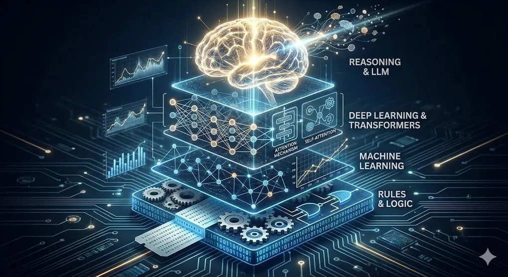
1. The Four Layers of AI

Before diving into architectures and algorithms, we need a map. AI isn’t one thing — it’s a stack of increasingly specialized technologies, each building on the previous layer:

               ┌───────────────────────┐
               │    LLM (2017→)        │  ← Most specialized
               │  Large Language Model  │
            ┌──┴───────────────────────┴──┐
            │    Deep Learning (2012)      │
            │   Multi-layer neural nets    │
         ┌──┴─────────────────────────────┴──┐
         │         ML (1990s)                 │
         │   Learning from data               │
      ┌──┴────────────────────────────────────┴──┐
      │              AI (1943→)                   │  ← Broadest foundation
      │   Any system that simulates intelligence  │
      └───────────────────────────────────────────┘

The key insight: understanding the lower layers gives you mastery over the upper ones. LLMs are built on Deep Learning, which is built on ML, which is built on the foundational ideas of AI. Skip a layer, and you’ll have blind spots that no amount of prompt engineering can fix.

1.1 Before AI Had a Name: Pre-1956

The story begins before “AI” even existed as a term:

• 1943 — Warren McCulloch & Walter Pitts published the first mathematical model of a neuron. Every neural network alive today is a descendant of this paper.
• 1950 — Alan Turing wrote “Computing Machinery and Intelligence” and proposed the Turing Test: can a machine fool a human into thinking it’s human?
• 1956 — At the Dartmouth Conference, John McCarthy coined the term “Artificial Intelligence.” AI became an academic discipline.
• 1958 — Frank Rosenblatt built the Perceptron — the first neural network that could actually learn from data.

1.2 The Two Schools of AI: Symbolism vs. Connectionism

This is the most fundamental ideological divide in AI’s history — and understanding it is the key to understanding why modern AI (Deep Learning) won.

	Symbolic AI (GOFAI)	Connectionism
Core belief	Intelligence = logical operations on symbols	Intelligence = emergent property of neural connections
Representatives	Expert systems, Knowledge graphs	Neural networks, Deep Learning
Method	Humans define rules (if-else)	Machines learn features from data
Why it failed	The world is too complex to enumerate all rules	—
Why it succeeded	—	Data + compute solved the “scale” problem

If you’re an RPA developer, pay attention: your RPA bots are quintessentially Symbolic AI — you explicitly write every rule, every condition, every exception handler. LLMs are the opposite extreme of Connectionism: nobody writes rules. The model learns from 45TB of text on its own.

This distinction explains everything that follows.

1.3 The AI Winters — and Why They Happened

AI’s history isn’t a straight line upward. It’s a story of two schools taking turns failing:

• First AI Winter (1974–1980): Minsky & Papert proved the Perceptron couldn’t solve XOR — Connectionism was humiliated. Funding dried up overnight.
• Symbolic AI takes over: In the 1980s, Expert Systems (rule-based AI) brought a renaissance. Companies invested millions.
• Second AI Winter (1987–1993): Expert Systems couldn’t scale. The bubble burst — Symbolism hit a dead end.
• Connectionism returns: In 2012, AlexNet crushed the ImageNet competition using a deep neural network, igniting the Deep Learning explosion. Connectionism won.

The pattern is clear: each “winter” happened when one school reached the limits of its approach. The question AI researchers kept asking — “Can we hand-craft enough rules?” — was ultimately answered with a resounding no.

1.4 Why Deep Learning Exploded in 2012

Three ingredients arrived simultaneously:

1. Data — ImageNet provided 14 million labeled images
2. Compute — NVIDIA GPUs made parallel matrix operations affordable
3. Algorithms — AlexNet (Krizhevsky et al.) proved that deeper networks with GPU training could demolish traditional methods

Remove any one of these, and the explosion doesn’t happen. This “three-body convergence” is also why it took 30 years from the Perceptron (1958) to practical Deep Learning (2012).

---

2. Machine Learning Core Theory

With the historical context in place, let’s build the mathematical foundation. Don’t worry — every formula comes with an intuition.

2.1 The Three Learning Paradigms

Type	Definition	Math	Real-world example
Supervised	Has labels (X, y) → learn f(X) ≈ y	min Σ L(f(xᵢ), yᵢ)	Invoice classification, fraud detection
Unsupervised	No labels X → find structure	Maximize P(X) or minimize reconstruction error	Customer clustering, anomaly detection
Reinforcement	Agent + Environment + Reward	max Σ γᵗrₜ	Game AI, robotics

The intuition: Supervised learning is like studying with an answer key. Unsupervised learning is like discovering patterns in a jigsaw puzzle without the box cover. Reinforcement learning is like training a dog — good behavior gets treats.

2.2 Loss Functions: Teaching Models What “Wrong” Means

A loss function measures how far the model’s prediction is from reality. Choose the wrong one, and the model learns the wrong lesson.

For regression (predicting continuous values):

$$L_{MSE} = \frac{1}{n} \sum_{i=1}^{n} (y_i - \hat{y}_i)^2$$

Intuition: “How far off am I, on average?” Squaring penalizes big errors disproportionately — being off by 10 is 100x worse than being off by 1.

For classification (predicting categories):

$$L_{CE} = -\sum_{i} y_i \log(\hat{y}_i)$$

Intuition: “How surprised am I by the correct answer?” If you predicted 99% confidence for the right class, -log(0.99) ≈ 0.01 (barely surprised). If you predicted 1%, -log(0.01) ≈ 4.6 (very surprised). The loss function punishes confident wrong answers harshly.

2.3 Gradient Descent: Finding the Bottom of the Mountain

Intuition: Imagine you’re blindfolded on a mountain. You can only feel the slope under your feet. To reach the valley, you take a step in the steepest downhill direction, then repeat.

That’s gradient descent: compute the gradient (slope) of the loss function with respect to each parameter, then update the parameters in the opposite direction.

$$w_{new} = w_{old} - \eta \cdot \nabla L(w)$$

Where η (learning rate) controls your step size:

Loss
  │╲
  │ ╲    ╱╲
  │  ╲  ╱  ╲    ← lr too large: bouncing over the optimal
  │   ╲╱    ╲
  │         ╲╱  ← Optimal solution
  └──────────── Iterations

  │╲
  │ ╲
  │  ╲
  │   ╲
  │    ╲•••••  ← lr too small: painfully slow convergence
  └──────────── Iterations

The evolution: SGD (one sample at a time) → Mini-batch SGD (small groups) → Adam (adaptive learning rate per parameter — the current default for most deep learning).

The Local Minima Myth

Here’s an insight that surprises most beginners:

The traditional worry is that SGD will get “stuck” in a local minimum — a valley that isn’t the deepest one. For low-dimensional problems, this is a real concern.

But in high-dimensional spaces — and LLMs operate in billions of dimensions — the landscape is fundamentally different. True local minima are astronomically rare. Instead, the real obstacles are saddle points: positions where the loss is a minimum in some directions but a maximum in others, like sitting on a horse saddle.

The good news? SGD naturally escapes saddle points because its inherent noise pushes it in random directions. This is one of the deep reasons why SGD works so well in practice, despite the theoretical difficulty of optimizing non-convex functions.

---

3. The Bias-Variance Tradeoff and Overfitting

This is the central dilemma of all machine learning — and one of the most important sections in this article.

3.1 Bias-Variance Decomposition

Every prediction error can be decomposed into three components:

$$\text{Error} = \text{Bias}^2 + \text{Variance} + \text{Irreducible Noise}$$

• Bias — The error from oversimplifying. The model is too simple to capture the true pattern → Underfitting.

  • In LLM terms: A model that’s too small produces incoherent, illogical responses. It simply lacks the capacity to model language properly.

• Variance — The error from overcomplicating. The model memorizes noise in the training data → Overfitting.

  • In LLM terms: The model “memorizes” training data verbatim. If you ask the exact same question from its training set, it recites the answer perfectly. Change one word in your question, and it falls apart.

Error
  │╲                    ╱
  │ ╲   Total Error   ╱
  │  ╲    ╱╲         ╱
  │   ╲  ╱  ╲•──────╱   ← Sweet Spot
  │    ╲╱    
  │   Bias²  ╲
  │           Variance
  └──────────────────── Model Complexity
     Simple ───────→ Complex

The art of machine learning is finding the sweet spot — complex enough to capture the real pattern, simple enough to generalize to new data.

3.2 Diagnosing Overfitting

The classic signal: training loss keeps going down, but validation loss starts going up.

Loss
  │
  │  ╱─── Validation Loss (starts rising)
  │ ╱
  │╱────── Training Loss (keeps falling)
  │
  └──────────────────── Epochs
         ↑
    Overfitting begins here

When you see this gap widening, the model is memorizing training data instead of learning generalizable patterns. Here’s your toolkit for fighting back:

3.3 The Eight Regularization Techniques

① L1 Regularization (Lasso)

$$L_{total} = L_{original} + \lambda \sum |w_i|$$

Intuition: “Tax every weight by its absolute value.” The bigger λ is, the heavier the tax. Some weights get driven to exactly zero — effectively performing automatic feature selection. The model learns to ignore irrelevant inputs.

② L2 Regularization (Ridge)

$$L_{total} = L_{original} + \lambda \sum w_i^2$$

Intuition: “Tax every weight by its square.” This doesn’t zero out weights, but pushes them all toward small values. The effect is spreading the model’s attention across all features rather than relying heavily on a few. This is mathematically equivalent to “Weight Decay” — the technique used in virtually every modern neural network.

🔧 Engineer’s Note: In production, L2 regularization is almost never implemented directly. Instead, it’s built into the AdamW optimizer as the weight_decay parameter. If you see weight_decay=0.01 in a training config, that’s L2 regularization. The “W” in AdamW literally stands for “Weight Decay done correctly” (decoupled from the gradient update).

③ Elastic Net (L1 + L2)

$$L_{total} = L_{original} + \lambda_1 \sum |w_i| + \lambda_2 \sum w_i^2$$

Combines the sparsity of L1 with the stability of L2. Best of both worlds.

④ Dropout (Srivastava et al., 2014)

During training, randomly turn off p% of neurons in each forward pass.

Training (p=0.5):
  ○──○──●──○      ● = turned off
  ○──●──○──○      Different each iteration
  ●──○──○──●

Inference:
  ○──○──○──○      All neurons active
  ○──○──○──○      Weights × (1-p)
  ○──○──○──○

Intuition: It’s like an implicit ensemble of exponentially many sub-networks. Each forward pass trains a different sub-network. At inference time, the full network acts as a vote of all these sub-networks. Typical values: 0.5 for hidden layers, 0.2 for input layers.

At inference, all neurons are active but weights are scaled by (1-p) to compensate — keeping the expected output the same.

🔧 Engineer’s Note: Modern LLMs (GPT-3+) actually don’t use Dropout — they rely on the massive dataset and other techniques for regularization instead. Dropout is still standard in smaller models and fine-tuning workflows.

⑤ Batch Normalization (Ioffe & Szegedy, 2015)

Normalize each mini-batch:

$$\hat{x} = \frac{x - \mu_B}{\sqrt{\sigma_B^2 + \epsilon}}$$

Then learn to rescale: $y = \gamma \hat{x} + \beta$ — where γ and β are trainable parameters.

Intuition: “Re-center and re-scale the data at every layer.” This stabilizes training, allows higher learning rates, and acts as implicit regularization. There’s still debate about the optimal placement: Conv → BN → ReLU vs Conv → ReLU → BN.

⑥ Early Stopping

Monitor validation loss. If it hasn’t improved for N consecutive epochs (the “patience” parameter), stop training and use the weights from the best epoch.

Intuition: “Stop studying before you start memorizing the textbook word-for-word.” Cost: zero. This is the simplest and most universally applicable regularization technique.

⑦ Data Augmentation

Create modified copies of your training data:

• Images: rotation, flipping, cropping, color perturbation
• Text: synonym replacement, back-translation, random deletion

Intuition: “Give the model more diverse examples so it can’t memorize any specific one.” This reduces variance by increasing the effective size of your training set.

⑧ Label Smoothing

Instead of hard labels [0, 0, 1, 0], use soft labels [0.033, 0.033, 0.9, 0.033].

Intuition: “Don’t let the model be 100% confident about anything.” This prevents extreme confidence in predictions and improves generalization — especially important in classification tasks.

3.4 Regularization Comparison

Technique	Compute cost	Effect on Bias	Effect on Variance	Best for
L1/L2	Low	Slight ↑	Significant ↓	All architectures
Dropout	Medium	Slight ↑	Significant ↓	FC > Conv layers
BatchNorm	Medium	Neutral	Moderate ↓	Conv / FC
Early Stopping	Zero	Slight ↑	↓	Everything
Data Augmentation	High	↓	Significant ↓	Images / Text
Label Smoothing	Low	Slight ↑	Moderate ↓	Classification

---

4. Inside the Neural Network

Now that we understand what we’re optimizing and how to prevent overfitting, let’s open the black box and look at the components.

4.1 Activation Functions

Without activation functions, a neural network — no matter how many layers — is just a linear transformation. Activation functions introduce non-linearity, allowing networks to model complex relationships.

Function	Formula	Pros	Cons
Sigmoid	σ(x) = 1/(1+e⁻ˣ)	Outputs 0-1, great for probabilities	Vanishing gradients, not zero-centered
Tanh	tanh(x)	Zero-centered	Vanishing gradients
ReLU	max(0, x)	Fast, mitigates vanishing gradients	Dead neuron problem
Leaky ReLU	max(αx, x)	Fixes dead neurons	α is a hyperparameter
GELU	x·Φ(x)	Standard in LLMs (GPT, BERT)	Slightly more expensive
Swish	x·σ(βx)	Smooth, self-gated	Slightly more expensive

The trend: Sigmoid → ReLU → GELU maps the evolution from classical neural nets to modern LLMs.

Why GELU Replaced ReLU in LLMs

ReLU has a hard cutoff at zero: any negative input becomes exactly 0. This creates two problems for language models:

1. Dead neurons: Once a neuron’s input goes negative, it outputs 0 and its gradient is 0 — it stops learning permanently
2. No gradient signal for near-zero values: ReLU is not smooth at x=0, creating a discontinuity

GELU (Gaussian Error Linear Unit) is a smooth approximation of ReLU that allows small negative values to pass through with reduced magnitude:

$$\text{GELU}(x) = x \cdot \Phi(x)$$

where Φ(x) is the cumulative distribution function of the standard normal distribution.

Intuition: instead of a hard gate (“on or off”), GELU acts like a soft gate (“how much should I let through?”). This smoothness gives the optimizer better gradient signals during training — critical when you’re training 175B parameters and every bit of gradient quality matters.

4.2 Backpropagation

Backpropagation is the algorithm that makes neural networks learnable. It applies the chain rule from calculus to compute gradients layer by layer:

$$\frac{\partial L}{\partial w} = \frac{\partial L}{\partial \hat{y}} \cdot \frac{\partial \hat{y}}{\partial z} \cdot \frac{\partial z}{\partial w}$$

Intuition: “If I wiggle this weight by a tiny amount, how much does the final loss change?” The chain rule lets us answer this for every weight in the network, even if it’s 100 layers deep.

The computation proceeds from the output layer backward to the input — hence “back-propagation.” The computational graph makes this systematic: each node stores its local gradient, and the chain rule multiplies them together from output to input.

4.3 The Gradient Problems

In deep networks, gradients must travel through many layers. Two things can go wrong:

Vanishing Gradients: As gradients multiply through many layers, they shrink exponentially. Layers near the input receive near-zero gradients and stop learning. This is why Sigmoid-based deep networks were impractical before 2012.

Solutions: ReLU (non-saturating gradients), Residual Connections (skip connections that bypass layers), BatchNorm (normalizing intermediate values).

Exploding Gradients: The opposite problem — gradients multiply and grow exponentially, causing weights to oscillate wildly.

Solutions: Gradient Clipping (cap the gradient norm), careful weight initialization (Xavier for Sigmoid/Tanh, He for ReLU).

---

5. Classic Architecture Evolution

Before the Transformer conquered everything, two families of architectures dominated different domains.

5.1 CNNs — Convolutional Neural Networks

The core idea: instead of connecting every input to every neuron (fully connected), use small sliding filters that scan across the input, detecting local patterns.

Why this matters:

• Parameter sharing: A 3×3 filter has only 9 parameters, regardless of image size → dramatically fewer parameters than fully connected layers
• Translation invariance: A cat is a cat whether it’s in the top-left or bottom-right of the image

The milestone architectures:

Year	Architecture	Key innovation
1998	LeNet-5	First practical CNN (digit recognition)
2012	AlexNet	Proved deep CNNs + GPU = state-of-the-art
2014	VGG	Deeper is better (16-19 layers)
2015	ResNet	Residual connections: y = F(x) + x
2019	EfficientNet	Scale width, depth, and resolution together

ResNet’s residual connection deserves special attention:

$$y = F(x) + x$$

Intuition: “If a layer can’t learn anything useful, at least let the data pass through unchanged.” The + x shortcut means the layer only needs to learn the residual (difference from identity). This seemingly simple trick solved the degradation problem — where adding more layers actually hurt performance — and enabled networks with 100+ layers.

5.2 RNNs → LSTM → GRU

For sequential data (text, time series, audio), we need networks with memory:

RNN (Recurrent Neural Network): Process one token at a time, passing a “hidden state” to the next step. Problem: the hidden state becomes a bottleneck. Information from 50 tokens ago is effectively forgotten — the vanishing gradient problem for sequences.

LSTM (Long Short-Term Memory, Hochreiter & Schmidhuber, 1997): Added three “gates” — Forget, Input, Output — that control what information to keep, add, or expose. The cell state acts as a highway for information to flow across many timesteps.

Intuition: think of LSTM as a conveyor belt. The cell state carries information forward. Gates are workers who decide what to add, remove, or read from the belt.

GRU (Gated Recurrent Unit): A simplified LSTM with only 2 gates instead of 3. Faster to train, similar performance.

The fatal limitation: RNNs process tokens sequentially — token 1, then token 2, then token 3. They can’t be parallelized. In an era of massive GPU clusters, this became unacceptable. Enter the Transformer.

5.3 Architecture Evolution Timeline

1943  McCulloch & Pitts → Mathematical neuron model
1950  Turing Test → "Can machines think?"
1956  Dartmouth Conference → AI is born
1958  Perceptron → First learnable network
1974  ❄️ First AI Winter
1986  Backpropagation → Training deep nets
1987  ❄️ Second AI Winter
1997  LSTM → Long-term memory for sequences
1998  LeNet-5 → First practical CNN
2012  AlexNet → Deep Learning explosion
2014  GAN / Dropout / GoogLeNet / VGG
2015  ResNet / Batch Normalization
2015  LSTM dominates NLP
2017  ⭐ Transformer → The game changer
2018  BERT / GPT-1
2019  GPT-2 ("too dangerous to release")
2020  GPT-3 (175B) / Scaling Laws
2022  ChatGPT → AI goes mainstream
2023  GPT-4 / Claude / Llama 2
2024  Claude 3.5 / GPT-4o / MoE / Open-source explosion
2025  Reasoning Models (o1/o3) / MCP / AI Agents
2026  Multi-Agent / AI enters enterprise core

---

5.5 Embeddings and Latent Space — The Portal from Discrete to Continuous

This is the most critical threshold for understanding modern AI.

Every formula that follows — Q·Kᵀ, Attention weights, cosine similarity — only makes sense once you understand this section. Without it, Transformers are pure magic. With it, they’re elegant engineering.

Why Do We Need Embeddings?

The problem: words are discrete symbols. “Cat” is just index 3421 in a vocabulary table. You can’t multiply “cat” by “dog.” You can’t compute the distance between “happy” and “joyful.”

The solution: map every discrete token into a continuous vector in high-dimensional space. Now “cat” isn’t index 3421 — it’s a vector of 12,288 numbers (in GPT-3’s case). And vectors support all the mathematical operations we need.

$$\text{"cat"} \xrightarrow{\text{Embedding}} [0.23, -0.15, 0.87, ..., 0.42] \in \mathbb{R}^{d}$$

Intuition: Embedding is the portal that takes language from the discrete world of symbols into the continuous world of mathematics. Once “meaning” becomes “geometry,” every tool in linear algebra becomes available.

Word2Vec (Mikolov et al., 2013)

The groundbreaking insight: “A word’s meaning is defined by its neighbors.”

Train a model to predict neighboring words in a large corpus (Skip-gram) or predict a word from its context (CBOW). The learned vector representations encode semantic relationships as geometric directions:

vector("King") - vector("Man") + vector("Woman") ≈ vector("Queen")

Why does this work? Because the “gender direction” in vector space is consistent across word pairs. The model didn’t learn a rule about gender — it discovered this geometric structure from millions of sentences.

The Geometry of Latent Space

Each word maps to a point in d-dimensional space. Semantic similarity becomes geometric proximity:

    Semantic geometry in high-dimensional space:

       Queen ●─────────────── King
             │                 │
       Gender direction       Gender direction
             │                 │
       Woman ●─────────────── Man
                 Gender axis

Key properties:

• Proximity: semantically similar words cluster together
• Direction: semantic relationships are encoded as vector directions (gender, tense, scale…)
• Arithmetic: vector operations correspond to meaning operations

GPT-3 uses d = 12,288 dimensions. That’s 12,288 axes along which every token is positioned — far too many to visualize, but the geometric principles hold.

Why Embeddings Are the Prerequisite for Transformers

Here’s the connection that unlocks everything:

• Self-Attention computes Q·Kᵀ — a dot product between vectors
• A dot product measures how aligned two vectors are — essentially cosine similarity
• If you don’t understand that words are already vectors in a geometric space, you can’t understand Q·Kᵀ

$$\text{Embedding} \xrightarrow{\text{§5.5}} \text{Geometry} \xrightarrow{\text{§6}} \text{Attention} \xrightarrow{\text{§7}} \text{Reasoning}$$

The Evolution of Embeddings

Method	Property	Limitation
Word2Vec / GloVe	Static: one vector per word	”bank” has same vector in “river bank” and “bank account”
ELMo	Contextualized via BiLSTM	Limited context window
BERT / GPT	Fully contextualized via Transformer	Context changes the vector at every layer

In modern Transformers, the embedding of “bank” is different in every sentence. The Attention mechanism (next section) is what makes this possible.

---

6. The Transformer — A Deep Dive

This is the most important section of this article. The Transformer architecture, introduced in the 2017 paper “Attention Is All You Need” (Vaswani et al.), is the engine inside every modern LLM. Understanding it is understanding modern AI.

6.1 Why the Transformer Was Needed

RNNs had two fatal problems:

1. Sequential bottleneck: Processing token-by-token meant no parallelization → painfully slow on GPU clusters
2. Long-range decay: Even LSTMs struggled with dependencies spanning hundreds of tokens

The Transformer’s core insight: replace recurrence entirely with Attention. Every token can directly attend to every other token — in parallel.

The Cost: O(n²) Complexity

This parallelism comes at a price. Self-Attention computes a similarity score between every pair of tokens, giving it O(n²) time and memory complexity where n is the sequence length.

Sequence length	Pairs computed	Relative cost
1,024 tokens	~1M	1×
4,096 tokens	~16M	16×
128,000 tokens	~16B	16,000×

This is why long Context Windows are so expensive — and why a 128K-context query costs dramatically more than a 1K-context query.

🔧 Engineer’s Note: In production, Flash Attention (Dao et al., 2022) solves this by restructuring the attention computation to be IO-aware — reducing memory reads/writes to GPU HBM. It doesn’t change the O(n²) math, but makes it 2-4× faster in practice. If you see “Flash Attention enabled” in a model config, this is what it means.

6.2 Self-Attention: Mathematics and Geometric Intuition

Core intuition: Attention is a “content-addressed” database query.

In a traditional database, you look up a key (exact match) to retrieve a value. In Attention, you use a query to compute “similarity” against all keys, then take a weighted average of all values. It’s a soft, differentiable lookup.

Step 1: Transform each input embedding X through three learned weight matrices:

• Q = X · Wq — Query: “What information am I looking for?”
• K = X · Wk — Key: “What information can I offer?”
• V = X · Wv — Value: “Here’s my actual content.”

Step 2: Compute attention:

$$\text{Attention}(Q, K, V) = \text{softmax}\left(\frac{QK^T}{\sqrt{d_k}}\right) \cdot V$$

Step 3: The geometric meaning of each operation:

Q · Kᵀ (dot product) — This is the heart of Attention. Geometrically, the dot product measures how aligned two vectors are — it’s a variant of cosine similarity (projection length × magnitude). Two vectors pointing in the same direction → large dot product → “highly relevant.”

Intuition: “How similar is my question (Q) to each key (K) in the room?”

÷ √dₖ (scaling) — Without this, high-dimensional dot products produce very large numbers. Large numbers push softmax into saturation (all mass on one token), causing vanishing gradients. Dividing by √dₖ keeps values in a trainable range.

Intuition: “Normalize so the model doesn’t become overconfident about a single token.”

softmax — Converts raw scores into a probability distribution (all weights sum to 1).

× V — Weighted average of all Value vectors, using attention weights. The output is a “mixture of all relevant information.”

Concrete example:

"The cat sat on the mat"

For the token "cat":
- attention to "sat" = 0.35  ← subject-verb relation (most similar direction)
- attention to "The" = 0.25  ← determiner
- attention to "mat" = 0.20  ← scene association
- attention to "on"  = 0.10
- attention to "the" = 0.10

→ New representation of "cat" = 0.35×V(sat) + 0.25×V(The) + 0.20×V(mat) + ...
→ This vector is no longer just "cat" — it's "cat in this context"

The Spotlight Metaphor

Here’s the classic example that shows why Attention matters:

"The animal didn't cross the street because it was too tired."

When the model reads "it", Attention decides where to shine the spotlight:
- "animal" ← attention = 0.72 💡 Spotlight ON (because "tired" refers to the animal)
- "street"  ← attention = 0.08    (streets don't get tired)

→ Through Attention, the model "understands" what the pronoun refers to
→ This is the core reason Transformers surpass RNNs

An RNN would struggle here — by the time it reaches “it,” the information about “animal” has decayed through many sequential steps. The Transformer’s Attention looks directly at every previous token, regardless of distance.

6.3 Multi-Head Attention

Why a single head isn’t enough

A single Attention head learns one set of (Q, K, V) projections — which means it can only look for one type of relationship at a time. But consider this sentence:

“The lawyer who drafted the contract reviewed it carefully.”

To fully understand “it,” the model needs to simultaneously track:

• Syntax: “it” is the object of “reviewed” (grammatical structure)
• Coreference: “it” refers to “contract,” not “lawyer” (semantic meaning)
• Proximity: “carefully” modifies “reviewed” (local context)

A single head can’t do all three at once — it’s forced to compromise.

The reading committee analogy

Think of Multi-Head Attention as assembling a reading committee. Instead of one person reading the document alone, you assign specialists:

• Head 1 (Grammarian): focuses on subject → verb → object structure
• Head 2 (Semanticist): focuses on meaning — what refers to what?
• Head 3 (Context Reader): focuses on nearby words and tone

Each specialist reads the same text but through their own lens (their own learned Q, K, V projections). Then they combine their notes into a single, richer understanding.

$$\text{MultiHead}(Q,K,V) = \text{Concat}(\text{head}_1, ..., \text{head}_h) \cdot W^O$$

where each head computes its own attention with its own learned projections:

$$\text{head}_i = \text{Attention}(QW_i^Q, KW_i^K, VW_i^V)$$

GPT-3 uses 96 attention heads — 96 different “specialists” analyzing every token relationship simultaneously. The final W^O projection learns how to best merge all 96 perspectives into a single output vector.

A pattern that scales beyond Transformers

Notice the core design principle here: specialized components working independently, then aggregating results outperforms a single generalist. This is the same principle behind Multi-Agent systems (covered in AI 06) — instead of one AI agent trying to handle everything, you deploy specialized agents (researcher, coder, reviewer) that collaborate. Multi-Head Attention is the token-level version of this idea; Multi-Agent is the system-level version.

6.4 Positional Encoding

Self-Attention treats its input as a set, not a sequence. Without positional information, “The cat sat on the mat” and “The mat sat on the cat” would produce the same result.

Solution: Add position information to each embedding using sinusoidal functions:

$$PE_{(pos, 2i)} = \sin\left(\frac{pos}{10000^{2i/d_{model}}}\right)$$ $$PE_{(pos, 2i+1)} = \cos\left(\frac{pos}{10000^{2i/d_{model}}}\right)$$

Intuition: “Give each position a unique frequency signature.” The sin/cos design allows the model to learn relative positions — the relationship between position 5 and position 10 is the same as between position 50 and position 55.

Modern alternatives include RoPE (Rotary Position Embedding) used by Llama and ALiBi — more efficient for long contexts.

6.5 Encoder-Decoder vs. Decoder-Only and Causal Masking

	Encoder-Decoder	Decoder-Only
Representatives	BERT, T5	GPT, Claude, Llama
Attention direction	Bidirectional	Causal (left-to-right only)
Best for	Understanding (NLU), Translation	Generation (NLG)
Why LLMs chose this	—	Natural autoregressive generation

Causal Masking — The Soul of GPT

The core distinction:

• BERT (Encoder): “I can see the entire sentence” → Great at understanding, but can’t generate
• GPT (Decoder): “I can only see what came before me” → Forced to learn to predict the next token

The mechanism: A mask matrix blocks attention to future tokens:

Causal Mask (lower triangular):

           The   cat   sat   on
  The    [  1     0     0     0  ]   ← "The" sees only itself
  cat    [  1     1     0     0  ]   ← "cat" sees "The", "cat"
  sat    [  1     1     1     0  ]   ← "sat" sees "The", "cat", "sat"
  on     [  1     1     1     1  ]   ← "on" sees everything before it

Masked positions (0) are set to -∞ before softmax → attention weight = 0

Why this matters: This mask means that during training, every position simultaneously learns to predict the next token. A sentence of N tokens generates N-1 training examples — extraordinarily efficient. This is the foundation of Generative Pre-training.

6.6 Feed-Forward Network & Layer Norm

Each Transformer block also contains:

• FFN: Two fully-connected layers with a GELU activation: FFN(x) = W₂ · GELU(W₁x + b₁) + b₂. This adds non-linearity and computational capacity beyond what Attention alone provides.
• Layer Norm (instead of Batch Norm): Normalizes across features for each token independently — better for variable-length sequences.
• Pre-Norm vs. Post-Norm: Pre-Norm (normalize before Attention/FFN) is now preferred — it produces more stable gradients in deep networks.

6.7 The Complete Transformer Block

Input Embedding + Positional Encoding
         │
    ┌────▼─────┐
    │ Multi-Head│
    │ Attention │
    └────┬─────┘
         │ + Residual Connection
    ┌────▼─────┐
    │ Layer    │
    │ Norm     │
    └────┬─────┘
         │
    ┌────▼─────┐
    │ Feed-    │
    │ Forward  │
    └────┬─────┘
         │ + Residual Connection
    ┌────▼─────┐
    │ Layer    │
    │ Norm     │
    └────┬─────┘
         │
    × N layers (GPT-3: N=96)

Stack 96 of these blocks, feed in 175 billion parameters, train on hundreds of billions of tokens — and you get GPT-3.

---

7. From Transformer to LLM

The Transformer is the engine. But turning that engine into ChatGPT requires several more critical innovations.

7.1 Tokenization

LLMs don’t process characters or words — they process tokens. A tokenizer splits text into subword units:

• BPE (Byte Pair Encoding): Used by GPT. Starts with individual characters, iteratively merges the most frequent pairs. “unhappiness” might become [“un”, “happiness”] or [“un”, “happ”, “iness”].
• SentencePiece: Used by Llama and multilingual models. Treats the input as raw bytes, making it language-agnostic.

Why tokenizer choice matters: the same sentence can be 15 tokens in one tokenizer and 30 in another — directly affecting model speed, cost, and context window usage.

7.2 The Paradigm Shift: Discriminative → Generative AI

This is the most important transition from 2012 (AlexNet) to 2022 (ChatGPT):

	Discriminative	Generative
Task	”Is this a cat or a dog?"	"Draw a cat” / “Write a story about a cat”
Math	Learn P(y|x) — predict label given input	Learn P(x) — model the data distribution, sample new instances
Representatives	CNN (ImageNet), SVM, XGBoost	GAN, VAE, GPT, Diffusion
Dominant period	2012–2020	2020–present

Why ChatGPT shocked the world: AI went from being a classifier (“I understand what this is”) to a creator (“I can make something new”). Next Token Prediction is fundamentally a generative task: model the probability distribution of language P(x), then sample from it.

Compression Is Intelligence (Ilya Sutskever)

But why can “just predicting the next word” produce reasoning ability?

Because to predict the next word accurately, the model must compress and understand the underlying patterns of reality. To predict what follows “The sun rises in the ___”, the model must effectively “understand” (compress into its weights) that the Earth rotates.

The most powerful compressor = the most powerful intelligence. This is also why Scaling Laws work: bigger models are better compressors.

7.3 Pre-training

The first stage of creating an LLM:

• Self-supervised learning: The model trains on raw text with a simple objective — predict the next token (Causal Language Model)
• Training data scale: Common Crawl, Wikipedia, Books, Code — hundreds of billions of tokens
• Compute cost: GPT-4 reportedly cost $100M+ to train

No human labels needed. The “labels” are the next token in every sentence — an essentially infinite supply of training signal from the internet.

7.4 The Bitter Lesson — The Philosophical Foundation of Scaling Laws

In 2019, Rich Sutton (a founding father of reinforcement learning) published a short essay that distills the entire history of AI into one uncomfortable truth:

“AI history teaches us that, in the long run, methods that leverage general-purpose compute (search and learning) always outperform methods that leverage human domain knowledge.”

What this explains:

• Past: Hand-crafted features (SIFT/HOG for vision), linguistic rules (parse trees for NLP), expert knowledge
• Present: Transformers removed all language-specific inductive biases — they rely purely on compute and data
• Result: “Brute force aesthetics” won — bigger models + more data = better results

Connecting back to §1.2: The Final Verdict on Symbolism vs. Connectionism

The arc of AI history is humanity repeatedly admitting that our hand-written rules can’t compete with what the machine learns on its own:

1. Computer Vision: Hand-designed features (SIFT, HOG) → replaced by CNNs
2. NLP: Hand-written grammar rules → replaced by LSTMs → replaced by Transformers
3. Training itself: Even the training objective simplified to Next Token Prediction

This is the final nail in Symbolism’s coffin — and a profound historical inevitability that §1.2 foreshadowed.

Why this is the philosophical foundation for Scaling Laws: If “compute always wins,” then the only rational strategy is to keep scaling. This explains why AI companies invest billions training ever-larger models — it’s not hype, it’s the Bitter Lesson playing out in real-time.

7.5 Scaling Laws (Kaplan et al., 2020)

The Bitter Lesson gets a mathematical formulation:

$$L(N) \approx \left(\frac{N_0}{N}\right)^{\alpha}$$

Where L = loss, N = parameter count, and N₀, α are empirical constants.

The key insight — log-log form:

$$\log L \approx -\alpha \cdot \log N + \text{const}$$

On a log-log plot, loss and parameter count form a straight line. This means: you don’t need to train a 100B model to predict its performance — train a few small models, draw the line, and extrapolate.

This applies equally to data size D and compute C:

$$L(N, D, C) \propto N^{-\alpha} \cdot D^{-\beta} \cdot C^{-\gamma}$$

Chinchilla Optimal (Hoffmann et al., 2022):

• Parameters and data should grow proportionally
• Chinchilla 70B (more data) beat Gopher 280B (more parameters)
• Conclusion: everyone had been training models that were “too big for their data”

7.6 RLHF and Alignment: Why ChatGPT?

The LLM training pipeline has three stages:

Stage 1: Pre-training
   Raw text → Next Token Prediction → Base Model
                                      (Can only "complete" text, doesn't understand dialogue)

Stage 2: SFT (Instruction Tuning)
   Instruction datasets → Supervised Fine-tuning → Instruct Model
                                                    (Learns "conversation mode")

Stage 3: RLHF
   Human preference rankings → Reward Model + PPO → Aligned Model
                                                     (Polite, safe, helpful)

• Reward Model: Humans rank multiple model responses → train a model to predict human preferences
• PPO (Proximal Policy Optimization): Use the reward model to fine-tune the LLM
• DPO (Direct Preference Optimization): A simpler alternative that skips the reward model

GPT-3 vs. ChatGPT: Same Engine, Completely Different Driving Experience

	GPT-3 (2020)	ChatGPT (2022)
Interface	API + complex prompts	Chat interface anyone can use
”How to make a bomb?”	Might continue: “…is a question many terrorists…"	"I can’t provide that information”
Nature	Text completion machine, no understanding of intent	”Tamed” dialogue engine
Users	Engineers, researchers	Everyone

Why ChatGPT — not GPT-3 — shocked the world:

• It wasn’t just a “big model” — it was the first model successfully “tamed” and fitted with a chat interface
• Alignment = teaching the model to understand what humans want, not just the most probable next token
• The product breakthrough mattered more than the technical breakthrough: ChatGPT let ordinary people control AI with natural language

7.7 Inference Techniques

How LLMs generate text at runtime:

• Temperature: Controls randomness. T=0 → greedy (always picks the most likely token). T=1 → full probability distribution. T>1 → more creative/random.
• Top-k sampling: Only consider the top k most likely tokens
• Top-p (Nucleus Sampling): Only consider tokens whose cumulative probability reaches p (e.g., 0.9)
• KV Cache: When generating token N+1, you don’t need to recompute Attention for tokens 1 through N — cache their K and V matrices
• Speculative Decoding: Use a small, fast model to draft multiple tokens, then verify with the large model in parallel — dramatically faster

7.8 Emergent Abilities: Why Now?

If Scaling Laws guarantee gradual improvement, why did AI seem to “explode” in 2022? This is where engineers feel like they’re witnessing magic — and understanding Emergence is the key to demystifying it.

Emergent Abilities

• Definition: Capabilities absent in small models that suddenly appear when the model exceeds a critical size threshold
• Controversy: Is this a true “phase transition,” or an artifact of evaluation metrics? (Schaeffer et al., 2023)

Concrete examples of emergence — “it just started working”:

Capability	Below threshold	Above threshold	Approximate threshold
3-digit arithmetic	Random accuracy (~0%)	>90% accuracy	~100B parameters
Chain-of-thought reasoning	Can’t follow multi-step logic	Solves step-by-step	~60B parameters
Code generation	Produces syntactically invalid code	Writes working functions	~60-100B parameters
Translation (unseen languages)	Gibberish	Coherent translation	~100B parameters

Why this feels like magic: You train a bigger model, and suddenly it can do things you never explicitly taught it. You didn’t add “arithmetic training data” — the model just figured it out from seeing enough text that happened to contain numbers.

Phase Transition: The Physics Analogy

Think of it like heating water. From 0°C to 99°C, water gets warmer — that’s “gradual improvement” (Scaling Laws). At 100°C, it suddenly boils — that’s emergence. The underlying physics (adding energy) is smooth, but the observable behavior changes discontinuously.

Capability
  │                        ╱╱ ← "Suddenly learned" (phase transition)
  │                      ╱
  │                    ╱
  │─────────────────╱
  │    "Parrot" phase       │
  │  (imitation only)       │
  └─────────────────────── Parameter count
         1B    10B   60B  100B+
                      ↑
                Emergence Threshold

Why now? Because hardware (GPU clusters) and data volume didn’t push models past the emergence threshold until 2020–2022. Before that threshold, models were sophisticated parrots — imitating text patterns. After it, they became reasoners — solving problems, writing code, analyzing data.

• GPT-2 (1.5B, 2019): “Too dangerous to release” — actually still quite weak
• GPT-3 (175B, 2020): Crossed the emergence threshold, but wasn’t “tamed”
• ChatGPT (2022): Emergence + Alignment + Product design = The explosion

The engineer’s takeaway: When evaluating an LLM for a task, don’t assume “slightly bigger = slightly better.” Some capabilities have hard thresholds. A 7B model that can’t do your task might need 70B — not 14B — to succeed.

7.9 Why Prompting Matters — The Mechanism Under the Hood

This section is the bridge from AI 00 to AI 01.

In-Context Learning (ICL)

The most mysterious ability of LLMs — one that overturns the traditional ML paradigm:

Traditional ML:
  [Large training dataset] → Gradient descent → Update weights w → New model

In-Context Learning:
  [Fixed LLM weights] + 3 examples in the Prompt → Direct inference
  The weights don't change at all! How does it "learn"?

In traditional ML, you train (update weights) then test (freeze weights). In ICL, the weights never change — yet the model adapts to new tasks just from a few examples in the prompt.

What Does a Prompt Actually Change?

Not the weights (W). The activation state (K, V).

Without a Prompt:
  The model wanders in "the universe of all possible text"
  → Could produce any style of output

With a Prompt (e.g., "You are a senior lawyer"):
  The Prompt fills the Transformer's K and V matrices
  → Attention's Q (Query) search range is "locked" to the subspace of
    "legal terminology and logic"
  → Output is narrowed to a specific domain

Full semantic space:
  ┌───────────────────────────────────┐
  │  Literature  Medicine  Law  Code  Finance  ... │ ← No Prompt: all open
  │           ┌────────┐                           │
  │           │  Law   │ ← "You are a lawyer"      │ ← Prompt narrows to subspace
  │           │subspace│                           │
  │           └────────┘                           │
  └───────────────────────────────────┘

The Theoretical Hypothesis

Research suggests ICL is essentially the Transformer performing implicit gradient descent during forward propagation (Akyürek et al., 2022; Von Oswald et al., 2023). The Attention layers, when reading the examples in your prompt, form a “temporary linear model” internally.

The Core Conclusion: Prompt = Programming in Natural Language

• You’re not “asking questions” — you’re setting the model’s initial state
• You’re not “typing input” — you’re programming, guiding the model to invoke knowledge from a specific region
• This is why changing a few words dramatically changes the output — because you’re moving the starting point of the search space
• → This is the entire theoretical foundation for AI 01: Prompt Engineering

But When Is Prompting Not Enough?

The K/V state that prompting changes is temporary and bounded by the Context Window. When you need to “permanently change model behavior” or “inject massive amounts of new knowledge,” prompting fails:

Problem 1: The model doesn’t know → Prompting can’t help

“What’s our company’s vacation policy?” → The LLM learned from public internet data. Your company’s internal policies aren’t in there. No amount of prompt engineering can conjure this information.

→ You need RAG (covered in AI 03)

Problem 2: The persona needs repeating every time → Prompting is tedious

Every conversation starts with “You are a professional financial analyst, please use IFRS terminology…” This works, but it’s wasteful and fragile.

→ You need Fine-tuning to make this the model’s default personality.

This leads directly to the LLM Customization Spectrum → §8.4

---

8. Model Selection and Customization

8.1 Major LLM Comparison (as of 2026)

Model	Organization	Parameters	Open-source	Strengths
GPT-4o	OpenAI	Undisclosed	✗	Multimodal, general capability
Claude 3.5	Anthropic	Undisclosed	✗	Long-form, code, safety
Gemini 2	Google	Undisclosed	✗	Multimodal, search integration
Llama 3.1	Meta	8B–405B	✓	Strongest open-source
Mistral	Mistral AI	7B–8x22B	✓	MoE architecture, efficient
Qwen 2.5	Alibaba	0.5B–72B	✓	Best open-source for Chinese
DeepSeek V3	DeepSeek	685B (MoE)	✓	Cost-effective, reasoning

8.2 Mixture of Experts (MoE): How Modern Models Cheat the Size vs. Cost Tradeoff

You may have noticed DeepSeek V3 has 685B parameters yet runs affordably. How? Because it doesn’t use all 685B parameters on every token — it uses Mixture of Experts (MoE).

Dense Model (e.g., Llama 70B):
  Every token → activates ALL 70B parameters → expensive

MoE Model (e.g., DeepSeek V3, 685B total):
  Every token → Router picks 2 out of 256 experts → activates ~37B parameters
  Total knowledge: 685B  |  Cost per token: ~37B  |  Best of both worlds

How it works:

1. The FFN layer in each Transformer block is replaced with N “expert” FFN layers
2. A lightweight Router network decides which 1-2 experts each token should use
3. Only the selected experts are activated → compute cost = 1 expert, not N

	Dense Model	MoE Model
Total parameters	70B	685B
Active per token	70B (100%)	~37B (~5%)
Knowledge capacity	Limited	Massive
Inference cost	High per param	Low per param
Examples	Llama 3.1, GPT-4(?)	Mistral 8x22B, DeepSeek V3

🔧 Engineer’s Note: MoE is why you’ll see “685B (MoE)” in model specs — the parenthetical matters enormously. A 685B MoE model might cost the same to run as a 70B dense model, while having the knowledge capacity of a much larger network.

8.3 How to Choose?

A simple decision tree: Privacy requirements → Open-source / Budget constraints → Smaller models or MoE / Chinese language → Qwen or DeepSeek.

8.4 The LLM Customization Spectrum: Prompt → RAG → Fine-tuning

This is the roadmap for the entire AI article series.

Level 3: Fine-tuning ── Change "model weights W"    ── Model's default personality
  │
Level 2: RAG ────────── Change "knowledge source"    ── Give the model what it doesn't know
  │
Level 1: Prompt ─────── Change "input / K,V state"   ── Guide model in the right subspace

Method	What it changes	Mechanism	Cost	Problem solved	Series article
Prompt Engineering	Input (K, V activation)	Narrow search subspace	Zero	”How to ask”	AI 01
RAG	Knowledge source	Embedding → Vector DB → inject Context	Medium	”Model doesn’t know”	AI 03
Fine-tuning	Model weights W	Gradient update on model parameters	High	”Model behavior/style”	—

How RAG Works (Preview of AI 03)

Your private data (internal docs, policies, reports)
     │
     ▼
Embedding Model → Convert text to vectors (recall §5.5)
     │
     ▼
Vector Database (Pinecone / Weaviate / Chroma)
     │  ← Store and index hundreds of thousands of vectors
     ▼
User asks question → Embed → Find K most similar documents in Vector DB
     │
     ▼
Retrieved documents + original question → Fed together into the LLM
     │
     ▼
LLM answers based on "retrieved real data", not memory guessing

• Embedding: Converts your private data into vectors — the same mathematical language the LLM speaks
• Vector Database: Stores and indexes vectors, enabling similarity search at scale
• RAG: Retrieve first, generate second — giving the LLM an “open-book exam” instead of a “closed-book exam”

When to Use What?

What's your problem?
  │
  ├─ "I don't know how to ask"          → Prompt Engineering (AI 01)
  │   Improve phrasing, add examples, structure
  │
  ├─ "The model doesn't know"           → RAG + Vector DB (AI 03)
  │   Internal docs, real-time data, private knowledge
  │
  └─ "The model's style is wrong"       → Fine-tuning
     Need specific tone, format, industry terminology

---

9. Model Evaluation Metrics

9.1 Traditional ML Metrics

• Accuracy: Overall correctness — but misleading for imbalanced datasets
• Precision / Recall / F1-Score: The tradeoff between “don’t miss any” (recall) and “don’t get any wrong” (precision)
• ROC-AUC: Model’s ability to discriminate between classes across all thresholds
• Confusion Matrix: Visualize where the model makes mistakes (type I vs. type II errors)

9.2 LLM-Specific Metrics

• Perplexity: The model’s average uncertainty about the next token. Lower perplexity = better language modeling. Intuition: “How surprised is the model by the actual next word?”
• BLEU / ROUGE: Measure text generation quality by comparing with reference texts
• MMLU / HumanEval / GSM8K: Standardized benchmarks testing knowledge, coding, and math reasoning

9.3 Human Evaluation

• Blind ranking (LMSYS Chatbot Arena): Humans compare two model outputs without knowing which model produced each
• LLM-as-Judge: Use a strong model (e.g., GPT-4) to evaluate other models’ output
• Why human evaluation remains irreplaceable: Metrics can’t fully capture helpfulness, safety, tone, and nuance. Real-world usefulness is ultimately judged by humans.

---

10. Future Outlook: What Comes Next?

10.1 Reasoning Models

OpenAI’s o1/o3 represent a paradigm shift: “Think before you answer.” Instead of generating tokens left-to-right, these models internalize Chain-of-Thought reasoning — spending more compute per query to produce more accurate answers.

From “fast thinking” (GPT-4) to “slow thinking” (o1). — echoing Daniel Kahneman’s System 1 vs. System 2.

10.2 Multimodal AI

The convergence of text + image + audio + video into unified models. GPT-4o, Gemini 2, and Claude already process multiple modalities. The end game: a single model that perceives the world the way humans do — through all senses simultaneously.

10.3 AI Agents

The shift from “answering questions” to “autonomously completing tasks.” Tool Use → MCP (Model Context Protocol) → Multi-Agent collaboration.

This is where LLMs go from being conversational partners to being autonomous workers — connecting to databases, calling APIs, managing workflows. We’ll cover this in depth in AI 04–06.

10.4 Open Questions

• Can hallucination be cured? Or is it inherent to probabilistic generation?
• Will Scaling Laws hit a wall? Data, energy, and compute constraints may impose limits
• How far away is AGI? The most contested question in AI. Opinions range from “2 years” to “never.”

---

11. Further Reading & Paper List

The papers that shaped modern AI, in chronological order:

1. Mikolov et al., 2013 — “Efficient Estimation of Word Representations in Vector Space” (Word2Vec)
2. Srivastava et al., 2014 — “Dropout: A Simple Way to Prevent Neural Network Overfitting”
3. Ioffe & Szegedy, 2015 — “Batch Normalization: Accelerating Deep Network Training”
4. He et al., 2015 — “Deep Residual Learning for Image Recognition” (ResNet)
5. Vaswani et al., 2017 — “Attention Is All You Need” (Transformer)
6. Sutton, 2019 — “The Bitter Lesson”
7. Kaplan et al., 2020 — “Scaling Laws for Neural Language Models”
8. Hoffmann et al., 2022 — “Training Compute-Optimal Large Language Models” (Chinchilla)
9. Ouyang et al., 2022 — “Training Language Models to Follow Instructions with RLHF”
10. Akyürek et al., 2022 — “What Learning Algorithm is In-Context Learning?”
11. Wei et al., 2022 — “Emergent Abilities of Large Language Models”

---

12. Key Takeaways

Let’s distill this entire journey into the insights that matter most:

1. LLM builds on DL, DL builds on ML, ML builds on AI — a stack of increasingly specialized technologies. Understanding the lower layers gives you mastery over the upper ones.

2. AI history = Symbolism vs. Connectionism. After two AI winters, Connectionism (neural networks) definitively won. Your RPA is Symbolism; LLMs are Connectionism’s ultimate expression.

3. Overfitting is ML’s central challenge. The eight regularization techniques — from L1/L2 to Dropout to Label Smoothing — each address it from a different angle.

4. Embeddings are the portal from discrete symbols to continuous mathematics. Without this transformation, nothing in modern AI works.

5. The Transformer’s Self-Attention is the engine of modern AI. Q·Kᵀ computes vector similarity (geometric projection); Causal Masking forces GPT to learn next-token prediction; Multi-Head Attention captures multiple relationship types simultaneously.

6. AI shifted from Discriminative to Generative — from “classify this” to “create something new.” This is why ChatGPT shocked the world.

7. Compression is Intelligence. Next Token Prediction forces the model to compress and understand the world’s patterns. The Bitter Lesson tells us: compute always beats hand-crafted rules.

8. Scaling Laws are historical inevitability. Log-log linearity means we can predict large model performance from small experiments. Chinchilla showed the importance of data-compute balance.

9. RLHF turned a text-completion engine into a conversation partner. The product breakthrough (chat interface + alignment) mattered as much as the technical breakthrough.

10. Prompt = programming in natural language. You’re not asking questions — you’re setting the model’s initial activation state, narrowing its search space. When prompting isn’t enough, RAG adds knowledge and fine-tuning changes behavior.

→ Next: AI 01: Prompt Engineering — Now that you understand why prompting works, learn how to do it effectively.