Apr 20, 2025

EBITDA Bridge Analysis: From Financial Statements to Actionable Insights

Financial Analysis EBITDA Waterfall Chart Python Power BI

What is an EBITDA Bridge?

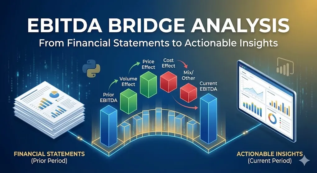
An EBITDA Bridge (also known as a Waterfall Chart or Walk) is a visualization technique used by analysts to decompose the change in a company’s EBITDA from one period to another into its fundamental drivers.

Why it matters: Instead of just saying “EBITDA dropped 23%,” a bridge chart answers why—was it pricing pressure, volume decline, cost inflation, or a mix of factors?

The Core Components

Component	What It Measures	Formula
Volume Effect	Impact of selling more/fewer units	ΔVolume × Prior ASP × Prior Margin
Price Effect	Impact of price changes	ΔASP × Current Volume
Cost Effect	Impact of COGS changes	ΔCOGS (at constant volume)
Mix Effect	Impact of product mix shifts	Residual after other effects
FX Effect	Currency translation impact	ΔRevenue due to exchange rates

[!NOTE] Understanding Mix Effect: Mix Effect captures the impact of product mix changes. If a company sells more high-margin products (e.g., iPhone Pro vs iPhone SE), EBITDA increases even with the same total volume. This is particularly important for multi-product companies like Apple, Samsung, or automakers with multiple vehicle lines.

When to Use EBITDA Bridge Analysis

Use Case	Example
Earnings Calls	”Our EBITDA grew $50M, driven by +$ 80M volume offset by -$30M pricing”
M&A Due Diligence	Decomposing target’s historical performance
Strategic Planning	Scenario analysis: “What if we raise prices 5%?”
Variance Analysis	Budget vs. actual performance decomposition

Building an EBITDA Bridge: Step-by-Step

Step 1: Gather the Data

You need two periods of data with these metrics:

Period 1 (Prior Year):
- Revenue, COGS, Opex, D&A, EBIT, EBITDA
- Volume (units sold)
- Average Selling Price (ASP) = Revenue / Volume

Period 2 (Current Year):
- Same metrics

Step 2: Calculate Each Effect

Volume Effect

volume_effect = (current_volume - prior_volume) * prior_asp * prior_gross_margin

Interpretation: How much EBITDA would change if only volume changed, holding price and costs constant.

Price Effect

price_effect = (current_asp - prior_asp) * current_volume

Interpretation: How much revenue changed due to pricing decisions.

Cost Effect

cogs_effect = prior_cogs - current_cogs  # Negative if costs rose
opex_effect = prior_opex - current_opex

[!TIP] Variable vs. Fixed Costs: When calculating Volume Effect, you should ideally use Variable COGS only. Including fixed costs in Volume Effect overstates the benefit of increased sales, since fixed costs don’t change with volume. For accurate analysis, separate your COGS into variable (materials, direct labor) and fixed (depreciation, rent) components.

D&A (Non-Cash Add-back)

da_effect = current_da - prior_da  # Positive = higher add-back

Step 3: Validate the Bridge

The bridge should “walk” from prior EBITDA to current EBITDA:

Prior EBITDA
  + Volume Effect
  + Price Effect
  + Cost Effect (COGS)
  + Cost Effect (Opex)
  + D&A Change
  ─────────────────
= Current EBITDA

Pro Tip: If there’s a residual, it’s typically captured as “Mix/Other” effect.

Python Implementation

import pandas as pd
import plotly.graph_objects as go

def calculate_ebitda_bridge(prior: dict, current: dict) -> pd.DataFrame:
    """
    Calculate EBITDA bridge components between two periods.
    
    Args:
        prior: Dict with keys: revenue, cogs, opex, da, volume
        current: Dict with same keys
    
    Returns:
        DataFrame with bridge components
    """
    # Derived metrics
    prior_asp = prior['revenue'] / prior['volume']
    current_asp = current['revenue'] / current['volume']
    prior_gross_margin = (prior['revenue'] - prior['cogs']) / prior['revenue']
    
    # Calculate effects
    volume_effect = (current['volume'] - prior['volume']) * prior_asp * prior_gross_margin
    price_effect = (current_asp - prior_asp) * current['volume']
    cogs_effect = prior['cogs'] - current['cogs']  # Negative = cost increase
    opex_effect = prior['opex'] - current['opex']
    da_effect = current['da'] - prior['da']
    
    # Prior & Current EBITDA
    prior_ebitda = prior['revenue'] - prior['cogs'] - prior['opex'] + prior['da']
    current_ebitda = current['revenue'] - current['cogs'] - current['opex'] + current['da']
    
    # Build bridge DataFrame
    bridge = pd.DataFrame({
        'Component': ['Prior EBITDA', 'Volume Effect', 'Price Effect', 
                      'COGS Impact', 'Opex Impact', 'D&A Change', 'Current EBITDA'],
        'Value': [prior_ebitda, volume_effect, price_effect, 
                  cogs_effect, opex_effect, da_effect, current_ebitda],
        'Type': ['start', 'delta', 'delta', 'delta', 'delta', 'delta', 'end']
    })
    
    return bridge


def plot_waterfall(bridge_df: pd.DataFrame, title: str = "EBITDA Bridge"):
    """Create a Plotly waterfall chart from bridge data."""
    
    fig = go.Figure(go.Waterfall(
        name="EBITDA",
        orientation="v",
        measure=bridge_df['Type'].map({'start': 'absolute', 'delta': 'relative', 'end': 'total'}),
        x=bridge_df['Component'],
        y=bridge_df['Value'],
        text=[f"${v/1e9:.1f}B" for v in bridge_df['Value']],
        textposition="outside",
        connector={"line": {"color": "rgb(63, 63, 63)"}},
        increasing={"marker": {"color": "#2ecc71"}},
        decreasing={"marker": {"color": "#e74c3c"}},
        totals={"marker": {"color": "#3498db"}}
    ))
    
    fig.update_layout(
        title=title,
        showlegend=False,
        template="plotly_white"
    )
    
    return fig

Case Study: Tesla FY2023

Let’s apply this framework to analyze Tesla’s 2023 performance, where aggressive price cuts made headlines.

The Data

Metric	FY2022	FY2023	Change
Deliveries	1.31M	1.81M	+38%
ASP	~$62,000	~$53,500	-14%
Revenue	$81.5B	$96.8B	+19%
EBITDA	$17.6B	$13.6B	-23%

The Bridge Analysis

Component	Impact	Interpretation
Prior EBITDA	$17.6B	Starting point
Volume Effect	+$30.7B	📈 Strong demand response to price cuts
Price Effect	-$15.4B	📉 14% ASP decline hit hard
COGS Impact	-$18.5B	📉 Costs rose faster than scale benefits
Opex Impact	-$1.7B	📉 SG&A growth
D&A Change	+$0.9B	📈 Non-cash add-back
Current EBITDA	$13.6B	Ending point

Key Insight

Volume gains (+ $30.7B) were almost entirely offset by price cuts (-$ 15.4B) and rising costs (-$18.5B).

Despite record deliveries of 1.8 million vehicles, EBITDA declined 23% year-over-year. The bridge reveals that Tesla’s pricing strategy was a bet on future cost reductions that hadn’t yet materialized.

👉 See the full interactive analysis: Tesla Pricing Strategy Impact Analysis

Power BI Implementation Tips

1. Use What-If Parameters for Scenario Analysis

// Create a "Price Scenario" parameter (-10% to +10%)
Adjusted_Price_Effect = 
    [Base_Price_Effect] * (1 + [Price Scenario Value])

Adjusted_EBITDA = 
    [Prior_EBITDA] + [Volume_Effect] + [Adjusted_Price_Effect] + [Cost_Effect]

2. Waterfall Chart Best Practices

Setting	Recommendation
Colors	Green = positive, Red = negative, Blue = totals
Labels	Show values in $M or$ B for readability
Sorting	Keep logical order (Volume → Price → Cost)
Subtotals	Add “Operating EBITDA” before non-cash items

Common Pitfalls to Avoid

Pitfall	Solution
Double-counting	Ensure Volume, Price, and Mix effects are mutually exclusive
Missing FX	Always isolate currency effects for multinational companies
Ignoring mix	Product mix shifts can mask true pricing power
Static costs	Separate fixed vs. variable costs for accurate volume effect

Summary

The EBITDA Bridge transforms opaque financial movements into a clear narrative:

Start with prior period EBITDA
Add volume effect (demand changes)
Add price effect (pricing power)
Subtract cost increases (or add savings)
Adjust for non-cash items (D&A)
Arrive at current period EBITDA

This framework is essential for:

Investment analysts decomposing earnings
FP&A teams explaining variances to executives
Strategy teams running scenario analyses

[!IMPORTANT] EBITDA vs. Cash Flow: Remember that EBITDA excludes D&A, CapEx, and Working Capital changes. While the EBITDA Bridge explains profitability drivers, you’ll often need a Cash Flow Bridge alongside it to understand where the money actually went. EBITDA can look healthy while cash flow suffers due to heavy capital expenditures or inventory buildup.