Everyone talks about prompting. But behind every prompt, behind every token prediction, behind every “GPT moment” — there are two ancient branches of mathematics quietly doing all the heavy lifting.

Linear Algebra gives AI the ability to compute in continuous space — measuring similarity, transforming representations, optimizing billions of parameters.

Discrete Mathematics gives AI the ability to handle symbols, structures, and logic — tokenizing language, building graph-structured networks, enforcing the rules of time.

But there is a silent third force that makes the entire enterprise learnable: Calculus. We convert discrete symbols into continuous vectors not because it’s convenient — but because it’s necessary. A discrete space has no slopes, no gradients, no way to answer the question “which direction is downhill?” Continuity is the price we pay for differentiability — and differentiability is the reason neural networks can learn at all. Every weight update in every training step is a tiny calculus operation: compute a gradient, follow it downhill, repeat billions of times. Linear algebra builds the space; calculus teaches the model how to navigate it.

Neither alone is sufficient. Together, they form the complete mathematical foundation of modern AI.

This article builds the intuition for why these two fields matter — not by teaching you textbook proofs, but by showing you exactly where each formula appears inside a Transformer, and what would break if you removed it.

---

Article Map

I — The Two Languages of Computing

1. The Sandwich Architecture — Discrete → Continuous → Discrete, and the cost of translation

II — Linear Algebra: The Continuous Engine 2. Vectors & High-Dimensional Space — Navigating 12,288 dimensions where humans can’t see 3. Dot Product, Projection & Cosine Similarity — How “meaning” becomes “geometry” 4. Matrix Multiplication — and Why It’s Not Enough — The linear trap, the non-linear escape, and residual highways 5. Transformation, Projection & Basis Change — Q, K, V as basis changes; Softmax as a differentiable switch; Positional Encoding

III — Discrete Math: The Structural Skeleton 6. Sets, Mapping & Space Complexity — Tokenization as discrete mapping; Quantization 7. Graph Theory — Neural networks as DAGs, Knowledge Graphs in RAG 8. Boolean Algebra & Causal Masking — The mathematics of “time flows forward”; Cross-Entropy & Training

IV — The Sacred Union 9. The Embedding Layer — Where Two Worlds Collide — The portal from symbols to vectors 10. Key Takeaways

---

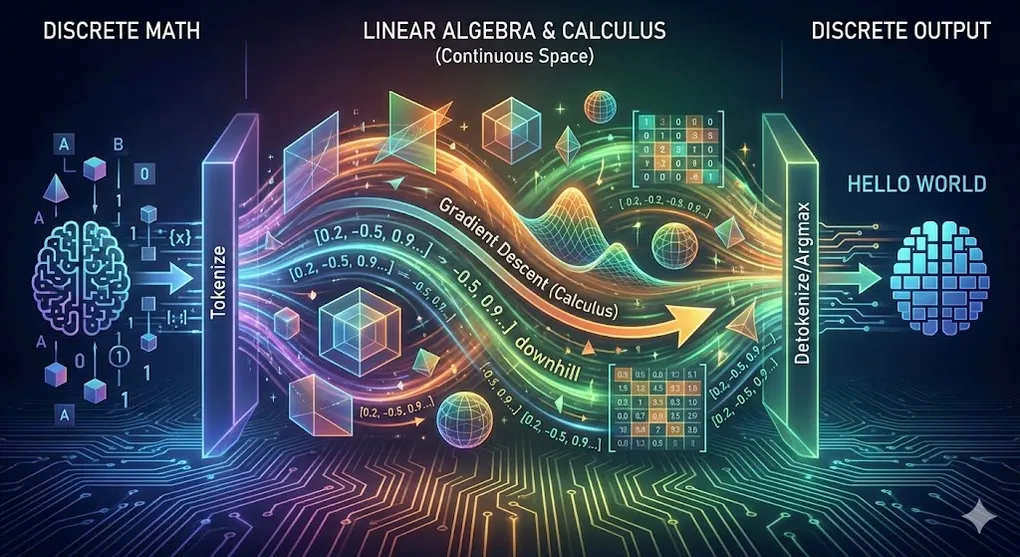
1. The Sandwich Architecture

Before we dive into formulas, we need to see the big picture. AI’s entire pipeline is a three-layer sandwich:

 Discrete                  Continuous                    Discrete
┌──────────┐          ┌──────────────────┐          ┌──────────────┐
│  "Hello   │  ──────→ │  [0.23, -0.15,   │  ──────→ │  "World"     │
│   World"  │ Tokenize │   0.87, ..., 0.42]│ argmax  │  (Token ID   │
│ (symbols) │ + Embed  │  96 layers of     │ / sample│   → decode)  │
│           │          │  matrix ops       │          │              │
└──────────┘          └──────────────────┘          └──────────────┘
 Discrete Math           Linear Algebra               Discrete Math
 governs this            governs this                 governs this

The core conflict: Human language is made of discrete symbols — letters, words, punctuation marks. You can’t take half of the letter “A.” You can’t compute the average of “cat” and “dog.” These symbols have no inherent mathematical structure.

But neural networks only operate on continuous numbers — floating-point vectors, differentiable functions, smooth gradients. They need to multiply, add, and differentiate everything.

This creates a fundamental translation problem. And translation is never free.

The Cost of Translation

Entry cost (Discrete → Continuous):

• Tokenization loss: “don’t” might become [“don”, “‘t”], severing semantic unity. “ChatGPT” might become [“Chat”, “G”, “PT”] — the model has to learn that these fragments form one concept.
• Embedding explosion: A vocabulary of 50,000 tokens × 12,288 embedding dimensions = 614 million parameters — and that’s just the translation layer, before a single Attention computation happens.

Exit cost (Continuous → Discrete):

• Information collapse: The model’s final hidden state is a rich 12,288-dimensional vector containing nuanced probability distributions. The moment we apply argmax or sampling to select one token, all that richness collapses into a single integer — a discrete choice. It’s an irreversible information bottleneck.

The philosophical implication: Every time you type a prompt and receive a response, the universe of continuous mathematics was summoned, marshaled through 96 layers of matrix operations, and then squeezed back through the narrow bottleneck of discrete symbols. Two entirely different branches of mathematics must cooperate seamlessly at both ends of this pipeline.

This is why understanding both is non-negotiable.

Note: The most critical component of this translation — the Embedding Layer — is so important that we’ve saved it for the finale in §9. It is the portal that makes the entire sandwich possible. But first, we must understand the two worlds it connects.

---

2. Vectors & High-Dimensional Space

Linear algebra begins with the simplest possible object: a vector — an ordered list of numbers.

$$\vec{v} = [v_1, v_2, v_3, ..., v_d]$$

In 2D, a vector is an arrow on a plane. In 3D, it’s an arrow in space. Your human visual intuition works fine here.

But GPT-3 operates in 12,288 dimensions. Llama operates in 4,096 dimensions.

Why these specific numbers? They aren’t random. 12,288 is the result of a specific architectural choice: 96 attention heads × 128 dimensions per head = 12,288. The “width” of the model is determined by how many parallel attention processes the engineers wanted to run. It’s not magic; it’s multiplication.

You cannot visualize 4,096-dimensional space. Nobody can. But this is precisely where linear algebra earns its keep — it provides a formal language for navigating spaces that no human mind can picture.

Why High Dimensions Actually Help

The common fear is the Curse of Dimensionality — in high-dimensional space, data points become sparse, distances lose meaning, and everything seems equally far from everything else.

But there’s a flip side that’s often overlooked: the Blessing of Dimensionality. In sufficiently high-dimensional space, concepts that overlap in low dimensions can be cleanly separated.

2D Space — "bank" is ambiguous:
 
   Financial ●────────────●  River bank
        (overlapping in 2D — can't separate them)

12,288D Space — "bank" splits into distinct regions:

   Dimension 1 (financial axis): Financial bank → high value
   Dimension 2 (geography axis): River bank → high value
   Dimension 47 (legal axis): Financial bank → moderate
   Dimension 893 (nature axis): River bank → high value
   ...
   
   → In 12,288 dimensions, these two meanings live in 
     completely different neighborhoods. No ambiguity.

Intuition: Think of dimensions as different lenses through which to examine a concept. With only 2 lenses, “bank” looks the same either way. With 12,288 lenses, the financial and geographical meanings light up completely different patterns — making them trivially distinguishable.

The Geometry of Meaning

In this high-dimensional space, proximity = similarity. Words with similar meanings cluster together, and the directions between clusters encode semantic relationships:

$$\vec{\text{King}} - \vec{\text{Man}} + \vec{\text{Woman}} \approx \vec{\text{Queen}}$$

This isn’t programmed — it’s discovered by the model from billions of sentences. The “gender direction” in vector space is consistent across word pairs because the model learned that “King” and “Queen” appear in analogous contexts, just as “Man” and “Woman” do.

The entire field of AI depends on this geometric property: meaning has direction. Without it, none of what follows — Attention, Cosine Similarity, Transformers — would work.

---

3. Dot Product, Projection & Cosine Similarity

Now that words are vectors in high-dimensional space, we need a way to measure how similar two vectors are. This is the single most important operation in modern AI.

The Dot Product: Two Meanings

The dot product of two vectors has a beautifully compact formula:

$$A \cdot B = \sum_{i=1}^{d} a_i \cdot b_i = \|A\|\|B\|\cos\theta$$

This single operation encodes two distinct geometric meanings:

Meaning 1: Directional Alignment (Angle)

Cosine Similarity isolates the angular component:

$$\text{cosine similarity} = \frac{A \cdot B}{\|A\|\|B\|} = \cos\theta$$

• $\cos\theta = 1$ → vectors point in the same direction → semantically identical
• $\cos\theta = 0$ → vectors are orthogonal → semantically unrelated
• $\cos\theta = -1$ → vectors point in opposite directions → semantically opposite

This is the formula that transforms the philosophical concept of “meaning” into the geometric concept of “angle.”

Meaning 2: Projection (Feature Capture)

The dot product also measures how much of vector A lies along the direction of vector B — the projection of A onto B:

$$\text{proj}_B A = \frac{A \cdot B}{\|B\|}$$

         A
        ╱|
       ╱ |
      ╱  |
     ╱   |          proj_B(A) = the "shadow" of A onto B
    ╱    |
   ╱     |
  ╱ θ    |
 ●───────●──────────→ B
 Origin   ↑
       Shadow of A on B
       (= dot product / ||B||)

Why this matters for AI: When a neural network computes $Q \cdot K^T$ in Self-Attention, it’s asking: “How much does each Key project onto my Query?” A large projection means that Key is highly relevant to what the Query is looking for. A small projection means irrelevance.

This is why the model can “capture specific features” — the dot product literally measures how much of a given feature direction is present in each vector.

The Deep Insight

$$\text{Semantic Similarity} = \text{Geometric Direction} = \cos\theta$$

This equation is the philosophical cornerstone of modern AI. It says: we don’t need to define “meaning” — we only need to measure angles in a space where meaning has been encoded as geometry.

---

4. Matrix Multiplication — and Why It’s Not Enough

If the dot product is AI’s basic measurement, matrix multiplication is AI’s basic operation. Every neural network layer performs:

$$y = Wx + b$$

Where:

• $x$ = input vector (e.g., a token’s embedding)
• $W$ = weight matrix (the learned parameters)
• $b$ = bias vector
• $y$ = output vector (the transformed representation)

What Matrix Multiplication Does Geometrically

Multiplying by a matrix $W$ performs a linear transformation — a combination of:

Operation	Geometric Effect	Example
Scaling	Stretch or compress along axes	Emphasize certain features
Rotation	Change the orientation	Reframe the representation
Reflection	Mirror across an axis	Invert a dimension’s meaning
Projection	Collapse to lower dimensions	Discard irrelevant information

Before W:                     After W (rotation + scaling):
   ↑ y                           ↑ y
   │    ● B                      │         ● B'
   │  ●  A                       │   ● A'
   │                              │
   └──────→ x                    └──────→ x
   
   W rotated and scaled the space — 
   A and B have a new relationship

Why GPUs Are AI’s Engine

A GPU is, at its core, a massively parallel matrix multiplication machine. A modern NVIDIA H100 can perform ~4,000 trillion floating-point operations per second (4 PFLOPS in FP8). When GPT-3 processes a single prompt through 96 layers of 12,288-dimensional matrix multiplications across 175 billion parameters — it needs every one of those PFLOPS.

This is why: without GPU = without AI. The 2012 Deep Learning explosion (§1.4 of AI 00) happened precisely when GPU compute became affordable enough to support large-scale matrix operations.

The Linear Trap: Why Matrix Multiplication Alone Fails

Here’s the critical insight that most explanations miss:

No matter how many linear layers you stack, the result is always equivalent to a single linear transformation.

$$W_n \cdot W_{n-1} \cdots W_2 \cdot W_1 = W_{\text{single}}$$

A thousand layers of matrix multiplication can be mathematically collapsed into one matrix. This means a purely linear network can only learn hyperplanes — flat decision boundaries. It can separate cats from dogs if they’re linearly separable. But most real-world problems aren’t.

The classic example: a purely linear network cannot solve XOR — the simplest non-linear classification problem. This was the exact critique that killed the Perceptron in 1969 and triggered the first AI Winter.

The Non-Linear Escape: Activation Functions

The solution: insert a non-linear activation function after every matrix multiplication.

$$y = \sigma(Wx + b)$$

Where $\sigma$ is a non-linear function like ReLU or GELU:

Function	Formula	Geometric Effect
ReLU	$\max(0, x)$	Hard gate: folds space along the zero-plane. All negative regions collapse to 0.
GELU	$x \cdot \Phi(x)$	Soft gate: smoothly attenuates negative values instead of hard-cutting.

ReLU: Hard fold                    GELU: Smooth fold
   y│       ╱                        y│        ╱
    │      ╱                          │      ╱
    │     ╱                           │    ╱
    │    ╱                            │  ╱·····  ← small negative values
    │   ╱                             │╱          pass through slightly
────┼──╱────── x                  ────┼──────── x
    │ 0 (hard cutoff)                 │  (smooth transition)

The intuition that unlocks everything:

• Matrix multiplication = rotating and scaling the canvas (a rigid, reversible transformation)
• Activation function = folding the paper (an irreversible, non-linear deformation)

With only rotation, you can reposition data but never create new separations. Once you fold, previously overlapping regions now live on different sides of the crease. Stack many fold-rotate-fold-rotate operations, and you can create arbitrarily complex decision boundaries.

This is why a neural network with non-linear activations is a universal function approximator — given enough parameters, it can learn any continuous function. Remove the activation functions, and you’re back to a single matrix multiplication, no matter how deep the network is.

🔧 Engineer’s Note: The evolution from ReLU to GELU mirrors the maturation of deep learning. ReLU (2012) was revolutionary for its simplicity and gradient-friendly properties, but its hard cutoff causes “dead neurons” — units that permanently output zero. GELU (2016, adopted universally in GPT/BERT) applies a smooth, probabilistic gate: $\text{GELU}(x) = x \cdot \Phi(x)$, where $\Phi$ is the Gaussian CDF. The smoothness gives the optimizer better gradient signals — critical when training 175 billion parameters.

Residual Connections — The Vector Highway

If activation functions solve the expressiveness problem, residual connections solve the depth problem. Why can GPT stack 96 layers of matrix operations without the signal degrading into noise?

The answer is deceptively simple:

$$y = F(x) + x$$

In plain English: instead of replacing the input with the layer’s output, add the output to the original input.

This + x creates a lossless shortcut — an information highway that bypasses the transformation entirely:

Without residual:                With residual:

x → [Layer] → F(x)              x ───┬──────────────────┐
                                  │                    │
If F is imperfect,               └→ [Layer] → F(x) ──(+)─→ F(x) + x
the original x is lost.                               │
96 imperfect layers             The original x survives
= signal destroyed.             no matter what F does.

Why this matters for the Discrete → Continuous theme:

The embedding vector x — the original continuous translation of a discrete token — survives intact through all 96 layers. Without residual connections, the continuous signal would degrade via the vanishing gradient problem: gradients shrink exponentially as they flow backward through many layers, making early layers untrainable.

With residual connections, gradients have a direct highway back to the input, bypassing all the matrix multiplications. This is why networks jumped from ~10 layers (pre-2015) to 96+ layers (modern Transformers) overnight.

🔧 Engineer’s Note: In PyTorch, a residual connection is a single line:

output = layer(x) + x  # That's it. The "+x" is the entire residual.

This one addition operation is arguably the most important architectural innovation since backpropagation. Without it, the 96-layer GPT stack would be untrainable — gradients would vanish long before reaching the early layers.

Normalization — Keeping the Signal on the Runway

Residual connections solve the gradient flow problem. But there’s a second stability crisis lurking inside deep networks: numerical drift.

After dozens of matrix multiplications, vector values can grow enormous (exploding activations) or shrink to near-zero (vanishing activations). Imagine a 12,288-dimensional vector passing through 96 layers of rotate-fold-rotate operations — without periodic recalibration, the numbers drift further and further from a usable range, like a plane gradually veering off the runway.

LayerNorm (original Transformer) and RMSNorm (Llama, Mistral) solve this by re-centering and re-scaling the vector after every sub-layer:

$$\text{LayerNorm}(x) = \frac{x - \mu}{\sigma} \cdot \gamma + \beta \qquad \text{RMSNorm}(x) = \frac{x}{\sqrt{\frac{1}{d} \sum x_i^2}} \cdot \gamma$$

In plain English: measure how “loud” the signal is (its variance, or its root-mean-square), divide by that volume to standardize it, then scale and shift by learned parameters ($\gamma, \beta$). Every layer’s output is pulled back to the center of the runway before takeoff into the next layer.

Without Normalization:           With Normalization:

Layer 1:  values ∈ [-1, 1]       Layer 1:  values ∈ [-1, 1]
Layer 10: values ∈ [-50, 50]     Layer 10: values ∈ [-1, 1]  ← re-centered
Layer 50: values ∈ [-10⁶, 10⁶]  Layer 50: values ∈ [-1, 1]  ← re-centered
Layer 96: NaN (overflow) 💀      Layer 96: values ∈ [-1, 1]  ← stable ✓

Normalization = "pull the data back to the center
                 of the runway after every layer"

Why this is the second guardian of depth: Residual connections preserve the gradient highway (backward pass). Normalization preserves activation stability (forward pass). Together, they are the two rails that let the 96-layer Transformer train without derailing.

🔧 Engineer’s Note: Modern Transformers (GPT-3, Llama) use Pre-Norm — applying normalization before Attention and FFN, not after. This subtle reordering makes training more stable at scale. In PyTorch:

# Pre-Norm Transformer block
x = x + attention(norm1(x))   # normalize, then attend, then add residual
x = x + ffn(norm2(x))         # normalize, then feed-forward, then add residual

RMSNorm (used by Llama/Mistral) drops the mean-centering step from LayerNorm, saving ~10% compute per layer with negligible quality loss. At 96 layers, that 10% adds up.

---

5. Transformation, Projection & Basis Change

We now have all the pieces to understand the most important operation in modern AI: Self-Attention. And the key to Attention is understanding what Q, K, V matrices really do.

The Basis Change Intuition

In linear algebra, a basis is a set of axes that define how you measure your space. The standard basis in 3D is (x, y, z) — but you could equally describe every point using a rotated set of axes (x’, y’, z’). The point hasn’t moved; you’ve changed the frame of reference.

Multiplying a vector by a matrix is a change of basis — viewing the same data through a different lens.

Q, K, V as Parallel Viewpoint Changes

In Self-Attention, each input embedding $X$ is projected through three different weight matrices simultaneously:

$$Q = XW_Q \quad \text{(Query: "What am I looking for?")}$$ $$K = XW_K \quad \text{(Key: "What can I offer?")}$$ $$V = XW_V \quad \text{(Value: "Here's my actual content.")}$$

Each matrix ($W_Q$, $W_K$, $W_V$) is a different basis change — transforming the same input into three different “viewpoints”:

Same input X = "bank"

         ┌────────────┐
         │   X · W_Q   │──→ Q: "bank" viewed through the
         │ (Query lens)│    "what-am-I-looking-for" frame
         └────────────┘
         
         ┌────────────┐
         │   X · W_K   │──→ K: "bank" viewed through the
         │  (Key lens) │    "what-can-I-offer" frame
         └────────────┘
         
         ┌────────────┐
         │   X · W_V   │──→ V: "bank" viewed through the
         │ (Value lens)│    "what-is-my-content" frame
         └────────────┘

Three different basis changes → three different perspectives
on the same token

Attention as Dynamic Basis Selection

The Attention formula brings it together:

$$\text{Attention}(Q, K, V) = \text{softmax}\left(\frac{QK^T}{\sqrt{d_k}}\right) \cdot V$$

Here’s what each step does geometrically:

1. $Q \cdot K^T$ — Compute the projection (§3) of each Query onto each Key. This measures: “From the Query’s viewpoint, how relevant is each Key?”

   💻 Code: scores = torch.matmul(Q, K.transpose(-2, -1))

2. $\div \sqrt{d_k}$ — Normalize so high-dimensional dot products don’t produce extreme values that saturate the softmax. When Softmax inputs are too large, the gradients approach zero, causing the model to stop learning (vanishing gradients).

   💻 Code: scores = scores / math.sqrt(d_k)

3. softmax — Convert raw relevance scores into a probability distribution (weights that sum to 1).

   💻 Code: attn_weights = F.softmax(scores, dim=-1)

4. $\times V$ — Take a weighted average of all Value vectors, using the attention weights. The output is a dynamically-constructed mixture of all relevant information.

The basis change insight: Attention doesn’t just compare tokens — it first re-frames each token into the most useful coordinate system for comparison (Q vs K), and then extracts information in yet another coordinate system (V). The model learns which basis changes are most useful during training.

This is why Attention is so powerful: it’s not a fixed comparison. It’s a learned, dynamic re-framing of the problem before every comparison. The model decides, for each token in each context, which viewpoint reveals the most relevant information.

🔧 Engineer’s Note: Multi-Head Attention (GPT-3 uses 96 heads) runs this entire process 96 times in parallel, each with different learned ($W_Q$, $W_K$, $W_V$) matrices. Each head learns a different basis change — one might specialize in grammatical structure, another in coreference, another in sentiment. The 96 perspectives are concatenated and merged through a final projection $W^O$. It’s 96 different lenses, combined into one image.

Softmax: The Differentiable Switch

Softmax deserves a closer look, because it is the critical bridge between the continuous and discrete worlds at the output of the model.

$$\text{softmax}(z_i) = \frac{e^{z_i}}{\sum_j e^{z_j}}$$

In plain English: exponentiate every score (amplifying differences), then divide by the sum so everything adds up to 1. The result is a probability distribution.

Softmax takes raw logits — continuous numbers that can be anything from $-\infty$ to $+\infty$ — and squeezes them into a probability distribution where every value is positive and the total is exactly 1. It is a continuous, differentiable approximation of a discrete choice.

Training vs. Inference — Two Different Uses of Softmax: During inference (generating text), Softmax acts as a decision switch — we sample or argmax from its output to pick one token. But during training, we never select a single winner. Instead, we treat the entire Softmax output as a probability landscape and compare it to the ground truth using Cross-Entropy (§8). The optimizer doesn’t just reward the correct token — it simultaneously punishes every incorrect token’s probability, sculpting the entire 100,000-dimensional distribution toward the target. This is why training requires a differentiable distribution (Softmax), not a hard choice (argmax) — and why the continuous nature of Softmax is essential for learning.

The Temperature dial — sliding between discrete and continuous:

$$P(x_i) = \frac{e^{z_i / T}}{\sum_j e^{z_j / T}}$$

In plain English: divide each score by Temperature T before exponentiating. T controls how “sharp” or “flat” the distribution is.

Temperature	Effect	Character
$T \to 0$	Distribution collapses to a one-hot vector (argmax)	Maximally discrete — one token gets 100%, rest get 0%
$T = 1$	Standard softmax	Balanced
$T \to \infty$	Distribution flattens to uniform	Maximally continuous — all tokens equally likely

Temperature is a control knob between the discrete and continuous worlds. Low temperature = rigid, deterministic, discrete selection. High temperature = fluid, random, continuous exploration. Every time you adjust the “creativity” slider in an AI chatbot, you’re turning this knob.

💻 Code:

# Standard softmax
probs = F.softmax(logits, dim=-1)

# Temperature-controlled softmax
# logits shape: [batch, vocab_size] (e.g., [1, 50257])
# T < 1: Differences magnified (Sharp) → strong tokens get stronger
# T > 1: Differences reduced (Flat) → weak tokens get a chance
probs = F.softmax(logits / temperature, dim=-1)

# T=0.1 → nearly deterministic (picks the top token)
# T=1.0 → balanced
# T=2.0 → creative and unpredictable

Temperature in practice — choosing the right setting for your task:

Task Type	Temperature	Rationale
Code generation	0.1–0.3	Code must be syntactically precise. One wrong bracket breaks everything. Low T forces the model to pick the most likely token (usually the correct one).
RAG / Q&A	0.2–0.5	Factual accuracy is critical. You want the model to stay close to retrieved context, not hallucinate creative alternatives.
Summarization	0.5–0.7	Some creativity helps with phrasing, but the core facts must stay intact.
Creative writing	0.8–1.2	Diversity and surprise are valuable. Higher T encourages the model to explore less common word choices, producing more varied prose.
Brainstorming	1.0–1.5	Maximum exploration. You want unexpected ideas, not the “obvious” answer.

This is why coding agents (GitHub Copilot, Cursor) default to low T (~0.2), while creative assistants (story generation, poetry) often use T > 1.0. The Temperature knob is a task-specific design choice — selecting how much you want the model to favor precision (discrete, deterministic) versus exploration (continuous, stochastic).

Positional Encoding — Injecting Discrete Order into Continuous Space

Self-Attention has a surprising flaw: it is permutation invariant. If you scramble the word order in a sentence, the raw attention scores are computed identically — each token attends to all others regardless of position. “The cat sat on the mat” and “mat the on sat cat The” produce the same attention weights.

This is catastrophic for language, where word order is meaning. The solution: add position information directly to the embedding vectors.

$$PE_{(pos, 2i)} = \sin\left(\frac{pos}{10000^{2i/d_{\text{model}}}}\right), \quad PE_{(pos, 2i+1)} = \cos\left(\frac{pos}{10000^{2i/d_{\text{model}}}}\right)$$

In plain English: each position is encoded as a set of sin/cos waves at different frequencies. Low dimensions oscillate fast (distinguishing neighboring words), high dimensions oscillate slowly (distinguishing distant words). Every position gets a unique “frequency fingerprint.”

Discrete position (integer):     Continuous signal (vector):

Position 0  ──────→  [sin(0), cos(0), sin(0), cos(0), ...]
Position 1  ──────→  [sin(1), cos(1), sin(0.0001), cos(0.0001), ...]
Position 2  ──────→  [sin(2), cos(2), sin(0.0002), cos(0.0002), ...]
   ...
Position n  ──────→  [unique frequency signature]

The sin/cos design encodes relative distances:
  distance(pos 5, pos 10) ≈ distance(pos 50, pos 55)

The Discrete → Continuous bridge: Position is inherently discrete (token 1, token 2, …). The sinusoidal encoding transforms this integer into a continuous vector that can be added to the embedding. The model then uses these positional signals during $Q \cdot K^T$ to distinguish “cat sat” from “sat cat.”

Modern alternative — RoPE (Rotary Position Embedding):

Llama, Mistral, and most modern LLMs use RoPE instead of sinusoidal encoding. RoPE encodes position as a rotation in the complex plane — directly applying the rotation matrices from §4:

$$R_\theta \cdot q = \begin{pmatrix} \cos(m\theta) & -\sin(m\theta) \\ \sin(m\theta) & \cos(m\theta) \end{pmatrix} \begin{pmatrix} q_0 \\ q_1 \end{pmatrix}$$

In plain English: treat each pair of embedding dimensions as a point on a 2D plane, then rotate it by an angle proportional to its position. The further back in the sequence, the larger the rotation.

Analogy: The Clock of Meaning

Imagine each pair of dimensions is a clock face. The token’s position determines where the hour hand points:

• Token at position 1: Hand points to 1 o’clock.
• Token at position 5: Hand points to 5 o’clock.

To find the relative distance between two tokens, you simply look at the angle difference between their hands. The angle between 1 o’clock and 5 o’clock is always 120 degrees — regardless of whether the hands are at (1, 5) or at (6, 10).

This is why RoPE is so powerful: it converts “distance” into “angle difference,” which the Dot Product naturally measures.

The brilliance: when you compute $Q \cdot K^T$ between a rotated Query at position $m$ and a rotated Key at position $n$, the rotation angles subtract, producing a result that depends only on the relative distance $(m - n)$. Absolute position becomes relative distance — purely through the algebraic property of rotation matrices.

🔧 Engineer’s Note: Positional encoding is the bridge between discrete math (integer positions) and linear algebra (continuous vectors). Without it, Transformers would treat language as a bag of words — losing all grammatical structure. With it, position is “baked into” the geometry of the vector space, allowing $Q \cdot K^T$ to capture both semantic and positional relevance simultaneously.

---

6. Sets, Mapping & Space Complexity

Now we cross from the continuous world to the discrete world. If linear algebra is the flesh and blood of AI, discrete mathematics is the skeleton — providing structure, boundaries, and logical rules.

Tokenization as Set Mapping

The first operation in any LLM pipeline is converting human text into numbers. This is a discrete mapping — a function from one finite set to another:

$$f: \text{Vocabulary} \to \mathbb{Z}^+$$ $$f(\text{"Apple"}) = 452, \quad f(\text{"Banana"}) = 893, \quad f(\text{"the"}) = 1$$

The vocabulary is a finite set — GPT-4 uses approximately 100,000 tokens. Every possible input must be decomposed into elements of this set. No token exists outside the set. This is the hard boundary of the discrete world.

BPE (Byte Pair Encoding) constructs this set algorithmically:

Step 1: Start with individual characters
  {"a", "b", "c", ..., "z", " ", ".", ...}

Step 2: Count most frequent adjacent pair in corpus
  "t" + "h" appears 9.2 billion times → merge into "th"

Step 3: Repeat thousands of times
  "th" + "e" → "the"
  "in" + "g" → "ing"
  "trans" + "former" → "transformer"

Final: A vocabulary of ~100K subword tokens

Space Complexity: The Vocabulary Tax

Here’s the discrete math insight most people miss: the size of your vocabulary set directly determines the size of your embedding matrix — and therefore a massive portion of your model’s parameters.

$$\text{Embedding Matrix Size} = |\text{Vocabulary}| \times d_{\text{model}}$$

Model	Vocabulary Size	Embedding Dim	Embedding Parameters	% of Total
GPT-2	50,257	768	38.6M	25%
GPT-3	50,257	12,288	617.6M	0.35%
Llama 2	32,000	4,096	131.1M	1.9%
GPT-4 (est.)	~100,000	~12,288	~1.23B	~0.07%

Observation: For smaller models (GPT-2), the embedding matrix is a quarter of all parameters — a massive discrete-math tax. For larger models, the proportion shrinks because the Transformer layers grow faster, but the absolute number (617M for GPT-3) is still enormous.

The tradeoff: A larger vocabulary means fewer tokens per sentence (more efficient encoding) but a larger embedding matrix (more parameters to train). A smaller vocabulary means more tokens per sentence (less efficient) but a leaner embedding matrix. This is a classic discrete optimization problem — and it’s why tokenizer design is a critical engineering decision.

🔧 Engineer’s Note: Multilingual models face this tradeoff acutely. Supporting Chinese, Japanese, Korean, Arabic, etc. can inflate the vocabulary to 250K+ tokens. SentencePiece (used by Llama, T5) treats input as raw bytes rather than characters, making it language-agnostic but potentially requiring more tokens to represent the same text in non-Latin scripts. The discrete math of set design ripples through the entire model’s efficiency.

🔧 Engineer’s Note — The OOM Killer (Out of Memory): The Embedding Table is often the first thing that crashes your GPU. The math is unforgiving:

Component	Calculation	VRAM
Weights (FP16)	100K × 12,288 × 2 bytes	2.4 GB
Gradients (FP16)	same size	2.4 GB
AdamW state 1 (FP32)	100K × 12,288 × 4 bytes	4.8 GB
AdamW state 2 (FP32)	same size	4.8 GB
Total for Embedding alone		~14.4 GB

That’s 14+ GB of VRAM consumed by a single lookup table — before any Attention or FFN computation begins. For reference, a consumer GPU (RTX 4090) has 24 GB total. This is why vocabulary size is a hardware architect’s nightmare: doubling $|V|$ doubles the Embedding Table’s memory footprint. It’s also why techniques like vocabulary pruning and parameter sharing (tying input/output embeddings) are critical in practice.

🔧 Engineer’s Note — Quantization: When Continuous Meets Reality: In theory, we want to compute with real numbers ($\mathbb{R}$) — infinite precision. In practice, GPUs have finite memory. Quantization compresses continuous floating-point weights into discrete, lower-precision formats:

Format	Bits	Precision	Use Case
FP32	32	Full	Training (gold standard)
FP16/BF16	16	Half	Training + inference
INT8	8	Low	Inference (2× speedup)
FP4/NF4	4	Very low	Edge deployment (4× compression)

This is the discrete world’s revenge on linear algebra. We take the smooth, continuous manifold of learned weights and force it onto a discrete grid with 256 steps (INT8) or just 16 steps (FP4). The result: models that run on a phone, at the cost of small precision errors (“quantization noise”).

# Quantize a model to 4-bit with bitsandbytes
model = AutoModelForCausalLM.from_pretrained(
    "meta-llama/Llama-2-7b",
    load_in_4bit=True  # Continuous → Discrete compression
)

The key insight: neural network weights follow a bell-curve distribution (most values near zero). Quantization exploits this — allocating more discrete levels near zero where the density is highest. This is why 4-bit quantization loses surprisingly little quality: the outlier values that suffer most from discretization are rare.

---

7. Graph Theory

If sets provide the elements of AI’s discrete world, graphs provide the connections.

Neural Networks Are Graphs

Every neural network is a Directed Acyclic Graph (DAG) — a graph where:

• Nodes = neurons (or layers, or operations)
• Edges = connections (weighted by learned parameters)
• Directed = information flows in one direction (input → output)
• Acyclic = no loops (in feedforward networks; RNNs are the exception)

A simple feedforward network as a DAG:

   Input Layer        Hidden Layer        Output Layer
   
   x₁ ●──────────→ h₁ ●──────────→ y₁ ●
       ╲          ╱    ╲          ╱
        ╲        ╱      ╲        ╱
         ╲      ╱        ╲      ╱
   x₂ ●──╲────╱──→ h₂ ●──╲────╱──→ y₂ ●
          ╱╲  ╱           ╱╲  ╱
         ╱  ╲╱           ╱  ╲╱
        ╱   ╱╲          ╱   ╱╲
   x₃ ●───╱──╲──→ h₃ ●───╱──╲──→ y₃ ●
          ╱    ╲          ╱    ╲
          
   Every edge has a learned weight w_ij
   Direction: strictly left → right (acyclic)

Why the DAG structure matters:

• Backpropagation works because the graph is acyclic — you can compute gradients layer by layer from output to input without circular dependencies.
• Topological sorting of the DAG determines the order of computation — the foundation of automatic differentiation in PyTorch/TensorFlow.
• If you accidentally create a cycle (a loop), gradient computation becomes undefined — the graph is no longer a DAG and standard backpropagation fails.

Self-Attention Is a Weighted Graph

Here’s the deeper connection to the core Transformer mechanism: Self-Attention is graph theory in action.

Every time the model computes attention, it is dynamically constructing a weighted, fully-connected graph where:

• Nodes = tokens in the sequence
• Edges = attention weights (the result of $\text{softmax}(Q \cdot K^T)$)
• Edge weights = how much token $i$ “pays attention to” token $j$

Input: "The cat sat on the mat"

Before Attention:                After Attention:
  Discrete tokens                  Weighted graph (values = attention weights)

  The  cat  sat  on  the  mat      The ──0.8──→ cat ──0.1──→ sat
                                    │ ╲                     ╱
                                  0.05╲ ╲──0.05──→ on ←──0.6
                                        ╲               ╱
                                         ╲──0.9──→ mat

  Each token attends to every other token with a learned weight.
  This is a dense, weighted, directed graph — regenerated dynamically
  for every forward pass, for every layer, for every sentence.

The graph theory insight: Attention doesn’t compare tokens in isolation. It constructs a complete graph (every node connected to every other node), assigns edge weights based on semantic relevance ($Q \cdot K^T$), and then uses those weights to aggregate information ($\text{weights} \times V$). This is message passing on a graph — a classic graph neural network (GNN) operation.

The Causal Mask (§8) is graph theory too: it removes edges from this graph. Without the mask, you get a fully-connected bidirectional graph (BERT). With the mask, you get a strictly lower-triangular graph where token $i$ can only attend to tokens $j \leq i$ (GPT).

🔧 Engineer’s Note: The connection to GNNs is not coincidental. Graph Attention Networks (GATs) explicitly use the same $Q \cdot K^T$ mechanism to weigh edges in an arbitrary graph. The Transformer is a special case where the graph is always fully connected (all tokens attend to all others), and the edge weights are learned rather than fixed by graph structure. This is why Transformers are sometimes called “graph neural networks on complete graphs.”

Knowledge Graphs in RAG

Graph theory also powers one of the most important augmentation techniques for LLMs: Knowledge Graphs.

In Retrieval-Augmented Generation (RAG), instead of stuffing raw text into context, you can organize knowledge as a graph where:

• Nodes = entities (people, concepts, companies)
• Edges = relationships (is-CEO-of, invented, belongs-to)

Knowledge Graph (subgraph):

   ┌──────────┐   invented    ┌─────────────┐
   │ Vaswani  │──────────────→│ Transformer  │
   └──────────┘               └──────┬───────┘
                                     │ powers
                                     ▼
   ┌──────────┐   is-built-on ┌──────────────┐
   │   BERT   │──────────────→│  Attention   │
   └──────────┘               └──────────────┘
        ↑                            ↑
        │ fine-tuned-from            │ uses
   ┌────┴─────┐               ┌─────┴────────┐
   │  GPT-1   │               │  Dot Product  │
   └──────────┘               └──────────────┘

Why graphs beat flat text: When a user asks “What mathematical operation does BERT rely on?”, the Knowledge Graph can traverse: BERT → is-built-on → Attention → uses → Dot Product. This structured traversal is more reliable than hoping the LLM finds this connection in a sea of unstructured text.

The discrete math insight: Graph traversal algorithms (BFS, DFS, shortest path) are classic discrete math. They don’t involve any calculus, any gradients, or any continuous optimization. They’re purely combinatorial — and they’re essential infrastructure for modern AI systems.

Two Graphs, Two Worlds

Although both Self-Attention and Knowledge Graphs use the language of graph theory, they operate on fundamentally different levels:

	Self-Attention Graph	Knowledge Graph (RAG)
Where	Inside the model (hidden computation)	Outside the model (external data structure)
Construction	Implicit — computed dynamically from $Q \cdot K^T$	Explicit — built by humans or extraction algorithms
Lifetime	Regenerated every forward pass, every layer	Persistent — lives in a database, survives between requests
Edges	Soft, continuous attention weights ∈ [0, 1]	Hard, discrete relationships (“invented”, “is-CEO-of”)
Purpose	Discover which tokens are relevant in context	Provide structured facts the model hasn’t memorized

How they work together in RAG: The Knowledge Graph (discrete, static) retrieves relevant facts via graph traversal (BFS, shortest path). These facts are injected into the prompt as text. The Transformer then builds its Self-Attention graph (continuous, dynamic) over the augmented context — weaving retrieved knowledge into its reasoning.

One graph lives in the world of discrete math. The other lives in the world of linear algebra. RAG is the pipeline that connects them.

---

8. Boolean Algebra & Causal Masking

The most elegant intersection of discrete math and AI is hiding in plain sight: the Causal Mask that makes GPT possible.

The Problem: Time Must Flow Forward

When GPT generates text, it predicts the next token based on only the previous tokens. It cannot look at the future — that would be cheating during training (you’d be predicting a word you’ve already seen).

But Self-Attention, by default, lets every token attend to every other token — including future ones. How do we enforce the arrow of time?

The Solution: An Upper Triangular Matrix of $-\infty$

Before the softmax in Self-Attention, we add a mask matrix — a discrete, binary object that encodes a simple Boolean rule: can_see(token_i, token_j) = (i ≥ j).

$$\text{Mask}_{ij} = \begin{cases} 0 & \text{if } i \geq j \quad \text{(allowed: present or past)} \\ -\infty & \text{if } i < j \quad \text{(forbidden: future)} \end{cases}$$

The Causal Mask for a 5-token sequence:

              Token₁  Token₂  Token₃  Token₄  Token₅
   Token₁  [   0      -∞      -∞      -∞      -∞   ]
   Token₂  [   0       0      -∞      -∞      -∞   ]
   Token₃  [   0       0       0      -∞      -∞   ]
   Token₄  [   0       0       0       0      -∞   ]
   Token₅  [   0       0       0       0       0    ]

   Lower triangle (0): "I can see you"    → attention flows
   Upper triangle (-∞): "I can't see you" → attention blocked

Why $-\infty$ instead of 0? Because of softmax:

$$\text{softmax}(z_i + (-\infty)) = \text{softmax}(-\infty) = \frac{e^{-\infty}}{\sum_j e^{z_j}} = \frac{0}{\sum_j e^{z_j}} = 0$$

Setting the mask to $-\infty$ guarantees that after softmax, the attention weight for future tokens is exactly zero — not “small,” not “nearly zero,” but mathematically, provably zero.

The Discrete Logic Inside Continuous Computation

This is the profound insight: inside a continuous, differentiable, gradient-friendly computation, we embed a perfectly discrete, Boolean logic gate.

The mask is not learned. It’s not optimized. It’s not a soft constraint. It’s a hard, binary rule — an if-else statement made of $-\infty$ values — that enforces the temporal structure of language.

The philosophical reading:

   Continuous math (Linear Algebra):
   "Every token can attend to every other token with any weight"
   
   Discrete math (Boolean Algebra):
   "NO. Time flows forward. You may NOT see the future."
   
   Result: The mask overwrites the continuous computation
   with a discrete structural constraint.
   
   This is discrete math carved into the heart of linear algebra.

The consequence: This single binary matrix is what makes GPT autoregressive — generating one token at a time, left to right, never peeking ahead. Remove the mask, and you get BERT (bidirectional, sees everything, great for understanding but can’t generate). Add the mask, and you get GPT (unidirectional, sees only the past, can generate new text).

The difference between the two most important architectures in AI history is one Boolean matrix.

🔧 Engineer’s Note: The Causal Mask is implemented efficiently as a triangular matrix operation, not as an element-by-element conditional:

# Generate the causal mask
mask = torch.triu(torch.ones(n, n), diagonal=1).bool()

# Apply: set forbidden positions to -infinity
scores = scores.masked_fill(mask, float('-inf'))

# After softmax, masked positions become exactly 0
attn_weights = F.softmax(scores, dim=-1)

The elegance: a single matrix addition enforces temporal causality across the entire sequence, with zero computational overhead beyond the addition itself.

The Inference Acceleration: KV Cache

The causal mask doesn’t just enforce logical correctness — it unlocks a massive engineering optimization that makes real-time generation possible.

The key insight: because the mask guarantees that token $i$ can never attend to token $i+1$, the Key and Value vectors for all previous tokens are frozen. They will never change, no matter what comes next. Past is immutable.

This means we don’t have to recompute $K$ and $V$ for the entire sequence every time we generate a new token. We store them once and reuse them:

Without KV Cache:                    With KV Cache:

Generate token 5:                    Generate token 5:
  Compute Q,K,V for tokens 1-5        Compute Q for token 5 only
  Full attention: 5×5 matrix           Attend to cached K,V of tokens 1-4
                                       Append new K₅,V₅ to cache

Generate token 6:                    Generate token 6:
  Compute Q,K,V for tokens 1-6        Compute Q for token 6 only
  Full attention: 6×6 matrix           Attend to cached K,V of tokens 1-5
                                       Append new K₆,V₆ to cache

Cost per step: O(N²)                 Cost per step: O(N) ✓
Total for N tokens: O(N³) 💀         Total for N tokens: O(N²) ✓

The discrete-continuous insight: A Boolean rule (“you cannot see the future”) guarantees mathematical immutability of past computations, which enables an engineering shortcut (caching) that transforms cubic cost into quadratic cost. Discrete logic creates the invariant; continuous computation exploits it.

🔧 Engineer’s Note: KV Cache is why long-context models consume so much VRAM during inference. For a 128K-token context in GPT-4 with 96 layers and 96 heads, the cache stores $128{,}000 \times 96 \times 96 \times 128 \times 2$ values (K and V) — potentially tens of gigabytes. This is the engineering tradeoff: memory for speed. Techniques like GQA (Grouped-Query Attention) — used in Llama 2 — reduce cache size by sharing Key/Value heads across multiple Query heads, cutting KV cache memory by 8× with minimal quality loss.

# Simplified KV Cache in generation loop
kv_cache = []
for token in generated_tokens:
    q = compute_query(token)           # Only the new token
    k, v = compute_key_value(token)    # Only the new token
    kv_cache.append((k, v))            # Append to cache
    all_k = concat([c[0] for c in kv_cache])  # All past Keys
    all_v = concat([c[1] for c in kv_cache])  # All past Values
    output = attention(q, all_k, all_v)        # Attend to full history

---

The Training Signal: Cross-Entropy — Where Continuous Predictions Meet Discrete Truth

We’ve seen how the model generates predictions (forward pass). But how does it learn? The answer lies at the intersection of our two pillars: the loss function.

During training, the model produces a continuous probability distribution over ~100,000 tokens. The correct answer is a discrete one-hot vector — a single token is right, all others are wrong.

$$L_{CE} = -\sum_{i} y_i \log(\hat{y}_i)$$

In plain English: cross-entropy measures “how surprised the model is by the right answer.” If the model assigned 99% probability to the correct token, surprise is low (loss ≈ 0.01). If it assigned 1%, surprise is high (loss ≈ 4.6). Training minimizes this surprise.

Model's prediction (continuous):    Ground truth (discrete):

  "the"    0.02                      "the"    0
  "cat"    0.85  ← high confidence    "cat"    1  ← correct answer
  "dog"    0.08                      "dog"    0
  "hat"    0.05                      "hat"    0
  
  Loss = -log(0.85) = 0.16 — low loss, model is learning well

The Discrete ↔ Continuous bridge in training: The truth is perfectly discrete (a single integer token ID). The prediction is perfectly continuous (a smooth probability distribution). Cross-entropy measures the “distance” between them, and backpropagation sends this error signal backward through all 96 layers, adjusting every weight matrix by computing gradients via the chain rule.

💻 Code:

# Forward pass: model outputs continuous logits
logits = model(input_ids)           # shape: (batch, seq_len, vocab_size)

# Loss: measure distance from continuous prediction to discrete truth
loss = F.cross_entropy(logits.view(-1, vocab_size), target_ids.view(-1))

# Backward pass: send gradient signal through the continuous pipeline
loss.backward()                     # Computes gradients for every parameter
optimizer.step()                    # Updates weights to reduce surprise

This is the training loop in three lines: continuous prediction, discrete truth, gradient correction. Every weight in the 175-billion-parameter model is adjusted to make the continuous output more closely match the discrete target.

---

9. The Embedding Layer — Where Two Worlds Collide

We’ve now built both pillars. This final section is the keystone that connects them — the most important data structure in modern AI.

The Portal

The Embedding Layer is the bridge between discrete mathematics and linear algebra.

Remember the discrete-continuous sandwich from §1? This is the moment we cross the crust and enter the filling.

It performs a deceptively simple operation:

$$\text{Input (Discrete)} \xrightarrow{\text{Table Lookup}} \text{Vector (Continuous)}$$

💻 Code:

# Define the bridge: 50,257 tokens × 12,288 dimensions
embedding = nn.Embedding(vocab_size=50257, embedding_dim=12288)

# Cross it: integer token ID → continuous vector
vector = embedding(torch.tensor([9246]))  # "Cat" → [0.12, -0.59, 0.88, ...]

Step by step:

1. User types:         "Cat"              ← Discrete symbol (human language)

2. Tokenizer maps:     "Cat" → 9246       ← Discrete mapping (§6)
                                             A set function: f(Cat) = 9246

3. Embedding lookup:   Row 9246 of a       ← The bridge: integer index → vector
                       giant matrix E
                       
4. Result:             [0.12, -0.59,       ← Continuous vector (linear algebra)
                        0.88, ..., 0.31]      Now we can compute dot products,
                        ∈ ℝ^12,288            cosine similarity, projections...

The Embedding Matrix: Where Discrete Meets Continuous

The embedding matrix $E$ is a lookup table stored as a matrix:

$$E \in \mathbb{R}^{|\text{Vocab}| \times d_{\text{model}}}$$

          d_model = 12,288 dimensions →
    ┌────────────────────────────────────────────┐
  0 │  0.02  -0.15   0.87  ...  0.31   0.19     │ ← "the"
  1 │  0.45   0.23  -0.56  ...  0.72  -0.11     │ ← "a"
  2 │ -0.33   0.67   0.12  ...  0.08   0.94     │ ← "is"
    │  ...                                       │
9246│  0.12  -0.59   0.88  ...  0.31  -0.22     │ ← "Cat" ★
    │  ...                                       │
50256│ -0.71   0.38   0.04  ...  0.55   0.18    │ ← last token
    └────────────────────────────────────────────┘
    
    50,257 rows (one per token in vocabulary)
    12,288 columns (one per dimension)
    
    Total: 617,558,016 parameters — just for this one matrix

The discrete math side: The row index (9246) comes from the tokenizer’s finite set mapping. It’s an integer. It obeys discrete rules (exact match, no interpolation — there is no token 9246.5).

The linear algebra side: The row content ($[0.12, -0.59, 0.88, ...]$) is a continuous vector. It lives in $\mathbb{R}^{12,288}$. It supports dot products, cosine similarity, matrix multiplication, gradient descent — every tool in the continuous optimization toolbox.

The bridge: A single row lookup transforms one into the other. This is the moment where discrete symbols become continuous geometry — where “Cat” stops being an arbitrary label and becomes a position in semantic space, measurable, comparable, and computable.

After the Bridge: Everything Is Linear Algebra

Once through the embedding layer, the discrete world is left behind. The subsequent 96 layers of Transformer computation — Self-Attention, Feed-Forward Networks, Layer Normalization — are pure linear algebra and calculus:

"Cat" (discrete)
    │
    ▼ Embedding Lookup (this section)
    │
 [0.12, -0.59, 0.88, ...] (continuous)
    │
    ▼ × W_Q, × W_K, × W_V (§5: basis change)
    │
    ▼ Q·Kᵀ / √d (§3: dot product / projection)
    │
    ▼ softmax → attention weights
    │
    ▼ × V → context-aware representation
    │
    ▼ Feed-Forward + GELU (§4: non-linear fold)
    │
    ▼ ... × 96 layers ...
    │
    ▼ Final logits → softmax → probability distribution
    │
    ▼ argmax / sample → Token ID 7891 (back to discrete!)
    │
 "Dog" (discrete again)

The full sandwich, mathematically:

$$\underbrace{\text{Token ID}}_{\text{Discrete (§6)}} \xrightarrow{E} \underbrace{\text{Vector}}_{\text{Continuous (§2-5)}} \xrightarrow{96 \text{ layers}} \underbrace{\text{Logits}}_{\text{Continuous}} \xrightarrow{\text{argmax}} \underbrace{\text{Token ID}}_{\text{Discrete}}$$

Discrete math handles the entry and exit. Linear algebra handles everything in between. The Embedding Layer is the portal that connects them.

---

10. Key Takeaways

1. AI is a sandwich: Discrete → Continuous → Discrete. Human language enters as symbols, gets processed as high-dimensional vectors, and exits as symbols again. Both ends are governed by discrete math; the middle is governed by linear algebra.

2. High-dimensional spaces are not a curse — they’re a feature. 12,288 dimensions let the model cleanly separate concepts that would be hopelessly tangled in 2D or 3D. Every additional dimension is another lens for disambiguation.

3. The Dot Product is AI’s most important operation. It encodes both directional similarity (cosine angle) and feature projection (shadow length). Self-Attention’s Q·Kᵀ is a massive parallel dot product — the engine of the Transformer.

4. Matrix multiplication alone is not enough. Without non-linear activation functions (ReLU/GELU), a thousand-layer network collapses to a single linear transformation. Non-linearity is what lets neural networks fold space and learn complex patterns.

5. Residual connections are the reason deep networks work. The simple addition y = F(x) + x creates a lossless highway that preserves the original signal through 96 layers. Without it, gradients vanish and deep Transformers are untrainable.

6. Q, K, V are basis changes — not just projections. Attention dynamically re-frames each token into three different viewpoints before comparing. The model learns the optimal viewpoints during training.

7. Softmax is the differentiable switch between worlds. It converts continuous logits into quasi-discrete probabilities. The Temperature parameter is a physical dial: turn it down for discrete certainty, turn it up for continuous exploration.

8. Positional Encoding is the discrete-continuous handshake. Transformers are order-blind by design. Sinusoidal waves and rotational matrices inject the discrete concept of “position” into the continuous vector space, making word order computable.

9. Vocabulary size is a discrete math constraint with continuous consequences. A 100K vocabulary × 12,288 dimensions = 1.23 billion parameters just for the lookup table. Tokenizer design is a critical engineering decision.

10. The Causal Mask is discrete logic inside continuous computation. A single Boolean matrix of 0 and $-\infty$ values enforces the arrow of time. It’s the difference between BERT (understands) and GPT (generates).

11. Cross-entropy bridges training: continuous predictions converge toward discrete truth. The loss function measures the distance between a smooth probability distribution and a one-hot target. Backpropagation sends the correction signal through the continuous pipeline.

12. The Embedding Layer is the sacred bridge. It transforms a discrete integer into a continuous vector — turning “Cat” from an arbitrary symbol into a point in geometric space. Without this bridge, none of modern AI works.

13. Not understanding discrete math → not understanding tokens, structures, or constraints. Not understanding linear algebra → not understanding similarity, training, or Attention. Both are required. Neither is optional. Together, they form the physical laws of the AI universe.