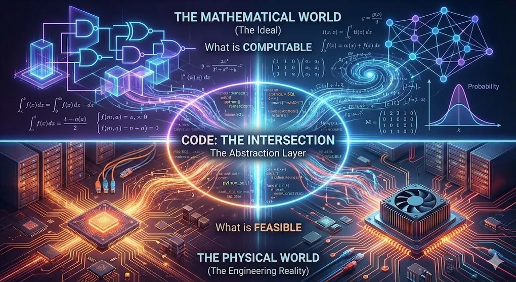
Every line of code you write sits at the intersection of two worlds:

The Mathematical World (the Ideal) — defines what is computable. Here, there is no time, no heat, no hardware. Only logic and truth.

The Physical World (the Engineering Reality) — defines what is feasible. Here, there are clock cycles, cache misses, memory walls, and the speed of light.

Most developers live in neither. They live in the comfortable abstraction layer of Python, JavaScript, or SQL — insulated from the math below and the silicon above. This works fine. Until it doesn’t.

When your model won’t converge, the answer is in calculus. When your query is inexplicably slow, the answer is in computer architecture. When your LLM hallucinates, the answer is in probability theory. When your distributed system silently corrupts data, the answer is in information theory.

This article builds the complete map — eight disciplines, organized into two tiers, showing exactly how they connect to the code you write every day.

---

Article Map

Part I — The Mathematical Foundations (what is computable)

1. Discrete Math — Logic, Graph Theory, Set Theory
2. Linear Algebra — Vectors, Matrices, Transformations
3. Calculus — Optimization, Gradient Descent, Physical Simulation
4. Probability & Statistics — Bayes, Monte Carlo, Stochastic Processes
5. Information Theory — Entropy, Compression, Channel Capacity

Part II — The Engineering Pillars (how to compute efficiently) 6. Computer Architecture — Memory Hierarchy, Cache, CPU vs GPU 7. Operating Systems & Networks — Scheduling, Concurrency, TCP/IP 8. Compilers — AST, Optimization, The Math-Hardware Interface

Part III — The Symphony 9. When All Eight Converge — 3D Games, ChatGPT, and the Full Stack in Action 10. Key Takeaways

---

Part I — The Mathematical Foundations

These five disciplines define the laws of physics of the digital universe. You can fight them, but you cannot break them.

---

1. Discrete Math — The Skeleton of Logic

One-line summary: It defines the structures a computer can understand.

A computer’s soul is discrete — 0 and 1. No fractions. No gradients. No “kind of true.” At the lowest level, everything is a choice between two states: on or off, yes or no, 1 or 0.

Discrete mathematics is the formal language for this binary world.

1.1 Logic — The Atomic Operation

Every computation — from a simple if statement to a trillion-parameter Transformer — decomposes into Boolean logic:

$$\text{AND}, \quad \text{OR}, \quad \text{NOT}, \quad \text{XOR}$$

These four operations, implemented as transistor gates in silicon, are the atoms of all computing. Your Python code, your SQL queries, your neural network — all compile down to sequences of these operations.

Why this matters beyond theory:

The Causal Mask inside GPT is a Boolean logic gate disguised as linear algebra. When GPT generates text, Self-Attention lets every token attend to every other token. But the model must not see the future — that would be cheating. The solution: multiply the attention scores by a mask matrix where:

$$\text{Mask}_{ij} = \begin{cases} 0 & \text{if } i \geq j \quad \text{(allowed: present or past)} \\ -\infty & \text{if } i < j \quad \text{(forbidden: future)} \end{cases}$$

Causal Mask for a 5-token sequence:

              Token₁  Token₂  Token₃  Token₄  Token₅
   Token₁  [   0      -∞      -∞      -∞      -∞   ]
   Token₂  [   0       0      -∞      -∞      -∞   ]
   Token₃  [   0       0       0      -∞      -∞   ]
   Token₄  [   0       0       0       0      -∞   ]
   Token₅  [   0       0       0       0       0    ]

   Lower triangle (0): "I can see you"    → attention flows
   Upper triangle (-∞): "You are my future" → attention = 0

After softmax, $e^{-\infty} = 0$ — the attention weight for future tokens is mathematically, provably zero. Not “small.” Zero.

The profound insight: Inside a continuous, differentiable, gradient-optimized computation, we embed a perfectly discrete, Boolean decision: see / don’t see. This single binary matrix is what makes GPT autoregressive. Remove it, and you get BERT. Add it, and you get GPT. The difference between the two most important architectures in AI history is one Boolean matrix.

🔧 Engineer’s Note: In PyTorch, the mask is typically created using torch.triu (upper triangular) and then filled with -inf:

mask = torch.triu(torch.ones(seq_len, seq_len), diagonal=1).bool()
attn_scores = attn_scores.masked_fill(mask, float('-inf'))

torch.triu(..., diagonal=1) produces the upper triangle of 1s (future positions). .masked_fill(mask, float('-inf')) then sets those positions to $-\infty$. One matrix addition enforces temporal causality across the entire sequence.

1.2 Graph Theory — The Topology of Connection

A graph is nodes + edges. It’s the simplest possible way to represent relationships — and it’s everywhere:

Domain	Nodes	Edges
Social networks	Users	Friendships
Internet	Servers	Links
Google Maps	Intersections	Roads
Neural networks	Neurons	Weighted connections
Knowledge Graphs	Entities	Relationships

Neural networks are Directed Acyclic Graphs (DAGs):

Input Layer        Hidden Layer        Output Layer

x₁ ●──────────→ h₁ ●──────────→ y₁ ●
    ╲          ╱    ╲          ╱
     ╲        ╱      ╲        ╱
x₂ ●──╲────╱──→ h₂ ●──╲────╱──→ y₂ ●
       ╱╲  ╱           ╱╲  ╱
      ╱  ╲╱           ╱  ╲╱
x₃ ●───╱──╲──→ h₃ ●───╱──╲──→ y₃ ●

Directed: information flows left → right only
Acyclic: no loops (critical for backpropagation)

Why DAG structure matters:

• Backpropagation requires acyclicity — gradients are computed via topological sort from output to input. A cycle would create circular gradient dependencies.
• Knowledge Graphs in RAG use graph traversal (BFS, DFS, shortest path) — purely discrete, combinatorial algorithms — to retrieve structured relationships that flat text search misses.

1.3 Set Theory — The Foundation of Data

SQL is set theory wearing a syntax costume:

SQL	Set Theory
SELECT	Projection (π)
WHERE	Selection (σ)
JOIN	Cartesian product + condition
UNION	Set union (A ∪ B)
INTERSECT	Set intersection (A ∩ B)
EXCEPT	Set difference (A \ B)

In AI, Tokenization is a set mapping:

$$f: \text{Vocabulary} \to \mathbb{Z}^+ \quad \text{where } f(\text{"Apple"}) = 452, \quad f(\text{"the"}) = 1$$

The vocabulary is a finite set — GPT-4 uses ~100,000 tokens. Every input must be decomposed into elements of this set. No token exists outside it. The finiteness of this set has enormous consequences (see §1.4).

1.4 Time and Space Complexity — The Price Tag

Discrete math doesn’t just define structures — it defines the cost of operating on them.

Space Complexity: The Vocabulary Tax

The size of your vocabulary set directly determines the size of your Embedding Matrix:

$$\text{Embedding Matrix} = |\text{Vocab}| \times d_{\text{model}}$$

Model	Vocab Size	Embedding Dim	Embedding Params	% of Total Model
GPT-2	50,257	768	38.6M	25%
GPT-3	50,257	12,288	617.6M	0.35%
Llama 2	32,000	4,096	131.1M	1.9%

For smaller models, the embedding matrix is a quarter of all parameters. This is the “vocabulary tax” — a discrete-math constraint with continuous consequences.

Time Complexity: The Attention Bottleneck

Self-Attention computes similarity between every pair of tokens, giving it O(n²) time and memory complexity:

Sequence Length	Pairs Computed	Relative Cost
1,024 tokens	~1M	1×
4,096 tokens	~16M	16×
128,000 tokens	~16B	16,384×

This is why a 128K-context query costs dramatically more than a 1K query. The O(n²) comes from a discrete counting argument — every token must attend to every previous token — but its consequences are felt in GPU memory and electricity bills.

🔧 Engineer’s Note: Flash Attention (Dao et al., 2022) doesn’t change the O(n²) asymptotic complexity — it restructures the computation to be IO-aware, minimizing reads and writes to GPU HBM (High Bandwidth Memory). The math is the same; the memory access pattern is radically different. Result: 2–4× wall-clock speedup from a pure engineering optimization, not a mathematical one. This is where §1 (math) meets §6 (architecture).

---

2. Linear Algebra — The Geometry of Data

One-line summary: It gives computers the ability to process multi-dimensional data — from 3D rendering to billion-parameter models.

When data has more than one dimension — and it almost always does — you need linear algebra. An image is a matrix. A word is a vector. A neural network is a sequence of matrix multiplications. GPU rendering is matrix transformation. PageRank is an eigenvector computation.

2.1 Vectors in High-Dimensional Space

A vector is an ordered list of numbers:

$$\vec{v} = [v_1, v_2, ..., v_d] \in \mathbb{R}^d$$

In 2D, it’s an arrow on paper. In 3D, it’s an arrow in space. In 12,288 dimensions (GPT-3’s embedding space), it’s a position in a space no human can visualize — but where linear algebra operates with perfect precision.

The Blessing of Dimensionality: High-dimensional spaces are counterintuitive. In 2D, “bank” (financial) and “bank” (river) overlap. In 12,288D, they occupy completely different neighborhoods. More dimensions = more axes to separate concepts along = less ambiguity.

2D — meanings overlap:     12,288D — meanings separate:

  Financial ●───● River       Dim 1 (financial): high | low
  (can't separate)            Dim 2 (geography): low  | high
                              Dim 47 (legal):    mod  | zero
                              ... 12,285 more separating axes ...

2.2 Dot Product, Projection & Cosine Similarity

The single most important operation in modern AI:

$$A \cdot B = \sum_{i=1}^{d} a_i b_i = \|A\|\|B\|\cos\theta$$

This encodes two geometric meanings:

① Directional Alignment (Cosine Similarity):

$$\text{cos\_sim}(A, B) = \frac{A \cdot B}{\|A\|\|B\|} = \cos\theta$$

• $\cos\theta = 1$ → same direction → semantically identical
• $\cos\theta = 0$ → orthogonal → unrelated
• $\cos\theta = -1$ → opposite → antonyms

Philosophical insight: This equation transforms “meaning” (a philosophical concept) into “angle” (a geometric concept). Semantic similarity is directional alignment.

② Projection (Feature Capture):

$$\text{proj}_B A = \frac{A \cdot B}{\|B\|}$$

         A
        ╱|
       ╱ |
      ╱  |
     ╱   |       proj_B(A) = the "shadow" of A onto B
    ╱ θ  |
   ╱     |
  ●──────●────────→ B
        Shadow

When Self-Attention computes $Q \cdot K^T$, it measures how much each Key projects onto the Query — how much of that feature direction is present. Large projection = highly relevant. Small projection = irrelevant.

2.3 Matrix Multiplication — and the Linear Trap

Every neural network layer computes:

$$y = Wx + b$$

Geometrically, multiplying by $W$ is a linear transformation — rotation, scaling, reflection, projection. GPUs exist because this operation is embarrassingly parallel — a modern H100 performs ~4 PFLOPS of matrix math per second.

The critical insight most explanations miss:

$$W_n \cdot W_{n-1} \cdots W_2 \cdot W_1 = W_{\text{single}}$$

Stack a thousand linear layers — mathematically, they collapse into one. A purely linear network can only learn flat hyperplanes. It cannot solve XOR. This is what killed the Perceptron in 1969.

The escape: non-linear activation functions.

$$y = \sigma(Wx + b)$$

Function	Effect	Intuition
ReLU: $\max(0,x)$	Hard fold at zero — all negatives become 0	Folding paper along a crease
GELU: $x \cdot \Phi(x)$	Smooth fold — small negatives pass through slightly	Bending paper in a smooth curve

• Matrix multiplication = rotating the canvas (rigid, reversible)
• Activation function = folding the paper (irreversible, non-linear)

Only the combination creates a universal function approximator — capable of learning any continuous function, given enough parameters.

2.4 Eigenvalues & Eigenvectors — The “Important Directions”

Beyond neural networks, linear algebra’s deepest concept is the eigenvector — the direction that a matrix transformation preserves:

$$Av = \lambda v$$

“When I multiply vector $v$ by matrix $A$, it doesn’t rotate — it just scales by $\lambda$.”

PageRank (Google’s founding algorithm) is an eigenvector computation: model the web as a matrix of links, find the dominant eigenvector, and that eigenvector is the ranking of pages by importance.

Principal Component Analysis (PCA) finds the eigenvectors of the covariance matrix — the “most important directions” in your data — enabling dimensionality reduction while preserving maximum variance.

2.5 Transformations, Q/K/V & Basis Change

In Self-Attention, each token is projected through three different weight matrices:

$$Q = XW_Q, \quad K = XW_K, \quad V = XW_V$$

Each matrix is a change of basis — viewing the same data through a different coordinate system:

Same input X = "bank"

  × W_Q → Q: "What am I looking for?" (Query frame)
  × W_K → K: "What information do I carry?" (Key frame)  
  × W_V → V: "What is my content?" (Value frame)

Three basis changes → three perspectives on the same token

The Attention formula:

$$\text{Attention}(Q, K, V) = \text{softmax}\left(\frac{QK^T}{\sqrt{d_k}}\right) \cdot V$$

Softmax deserves special attention: it takes raw scores (logits) of any range $(-\infty, +\infty)$ and compresses them into a probability distribution where all values are positive and sum to exactly 1:

$$\text{softmax}(z_i) = \frac{e^{z_i}}{\sum_j e^{z_j}}$$

Intuition: Softmax is a normalizing amplifier. It exponentiates the scores (amplifying differences — a score of 10 becomes vastly more dominant than a score of 5), then normalizes so they sum to 1. The result: the model allocates its “attention budget” as a probability distribution, concentrating focus on the most relevant tokens.

The basis change insight: Attention doesn’t just compare tokens — it first re-frames them into learned coordinate systems (Q vs K), computes relevance via dot product, normalizes via softmax, then extracts content in yet another frame (V). The model learns which re-framings are most useful.

2.6 Positional Encoding — Injecting Discrete Order into Continuous Vectors

Self-Attention has a surprising property: it’s permutation invariant. If you scramble the word order in a sentence, the attention scores are computed identically (each token attends to all others regardless of position). “The cat sat on the mat” and “mat the on sat cat The” would produce the same attention weights.

This is catastrophic for language — word order is meaning. The solution: add position information directly to the embedding vectors.

$$PE_{(pos, 2i)} = \sin\left(\frac{pos}{10000^{2i/d_{\text{model}}}}\right), \quad PE_{(pos, 2i+1)} = \cos\left(\frac{pos}{10000^{2i/d_{\text{model}}}}\right)$$

In plain English: each position is converted into a set of sin/cos waves at different frequencies. Low dimensions oscillate fast (distinguishing neighboring words), high dimensions oscillate slowly (distinguishing distant words). Every position thus gets a unique “frequency fingerprint.”

Discrete position (integer):     Continuous signal (vector):

Position 0  ──────→  [sin(0), cos(0), sin(0), cos(0), ...]
Position 1  ──────→  [sin(1), cos(1), sin(0.0001), cos(0.0001), ...]
Position 2  ──────→  [sin(2), cos(2), sin(0.0002), cos(0.0002), ...]
   ...
Position n  ──────→  [unique frequency signature]

Each position gets a unique "fingerprint" in continuous space.
The sin/cos design encodes relative distances:
  distance(pos 5, pos 10) ≈ distance(pos 50, pos 55)

The discrete → continuous bridge: Position is inherently discrete (token 1, token 2, …). The sinusoidal encoding transforms this integer into a continuous vector that can be added to the embedding. The model then uses these positional signals during attention to distinguish “cat sat” from “sat cat.”

Modern alternatives: RoPE (Rotary Position Embedding, used by Llama) encodes position as a rotation in vector space — an elegant application of rotational matrices from linear algebra. ALiBi adds a linear bias to attention scores based on distance — simpler and more efficient for long contexts.

🔧 Engineer’s Note — RoPE and the Geometry of Position: RoPE (Su et al., 2021), now standard in Llama, Mistral, and most modern LLMs, deserves special attention because it connects §2’s rotation concept directly to positional encoding. Instead of adding a positional vector to the embedding (as sinusoidal PE does), RoPE rotates the Query and Key vectors by an angle proportional to their position:

$$R_\theta \cdot q = \begin{pmatrix} \cos(m\theta) & -\sin(m\theta) \\ \sin(m\theta) & \cos(m\theta) \end{pmatrix} \begin{pmatrix} q_0 \\ q_1 \end{pmatrix}$$

In plain English: treat each pair of dimensions in the Query vector as a point on a 2D plane, then rotate that point by a fixed angle determined by its position in the sentence. The further back in the sequence, the larger the rotation.

This is the exact 2D rotation matrix from §2.3 — the same operation used in 3D rendering and physics engines, now repurposed to encode position in a sentence. The brilliance: when you compute $Q \cdot K^T$ between a rotated Query at position $m$ and a rotated Key at position $n$, the rotation angles subtract, producing a result that depends only on the relative distance $(m - n)$, not the absolute positions. Absolute position information (rotation) is transformed into relative position information (angle difference) — purely through the algebraic property of rotation matrices. This is why RoPE generalizes to longer sequences than it was trained on: the relative geometry is preserved regardless of absolute position.

The Complex Plane Connection: The deepest way to understand RoPE is through the complex plane. Each pair of embedding dimensions $(q_0, q_1)$ is treated as a complex number $q_0 + q_1 i$. Euler’s formula tells us:

$$e^{i\theta} = \cos\theta + i\sin\theta$$

Multiplying a complex number by $e^{im\theta}$ is a rotation by angle $m\theta$ — this is exactly what the rotation matrix above does, but expressed more elegantly. Now, the dot product of two rotated vectors at positions $m$ and $n$ becomes:

$$q \cdot e^{im\theta} \times \overline{k \cdot e^{in\theta}} = q \cdot \bar{k} \cdot e^{i(m-n)\theta}$$

In plain English: on the complex plane, “rotation” is simply “multiplication by a unit complex number.” When two rotated vectors are dot-producted, the angles naturally subtract, leaving only the relative position $(m-n)$. This is why RoPE can use “absolute rotations” to capture “relative distances” — the algebraic property of complex multiplication does it automatically.

🔧 Engineer’s Note: Positional encoding is the bridge between discrete math (integer positions) and linear algebra (continuous vectors). Without it, Transformers would treat language as a bag of words — losing all grammatical structure. With it, position is “baked into” the geometry of the vector space, allowing Q·Kᵀ to capture both semantic and positional relevance simultaneously.

---

3. Calculus — The Engine of Change

One-line summary: It lets computers simulate the physical world and learn from mistakes.

Discrete math handles states. Linear algebra handles spaces. Calculus handles change — how things move, grow, shrink, and optimize over time.

3.1 Optimization — Finding the Bottom of the Mountain

The central problem of machine learning: find the parameters $w$ that minimize a loss function $L(w)$.

Gradient Descent uses the derivative to find the direction of steepest descent:

$$w_{\text{new}} = w_{\text{old}} - \eta \cdot \nabla L(w)$$

Intuition: You’re blindfolded on a mountain. You feel the slope under your feet (the gradient). You step in the steepest downhill direction. Repeat.

Loss
  │╲
  │ ╲    ╱╲
  │  ╲  ╱  ╲    ← η too large: bouncing over the optimal
  │   ╲╱    ╲
  │         ╲╱  ← Optimal solution
  └──────────── Iterations

  │╲
  │ ╲
  │  ╲
  │   ╲
  │    ╲•••••  ← η too small: painfully slow convergence
  └──────────── Iterations

Why calculus is non-negotiable: Without derivatives, there is no gradient. Without gradients, there is no learning. Without learning, there is no AI. The chain rule — calculus’s most important theorem — makes backpropagation possible:

$$\frac{\partial L}{\partial w} = \frac{\partial L}{\partial \hat{y}} \cdot \frac{\partial \hat{y}}{\partial z} \cdot \frac{\partial z}{\partial w}$$

“If I wiggle this weight by a tiny amount, how much does the final loss change?” The chain rule answers this for every weight in the network, even if it’s 96 layers deep.

3.2 The Saddle Point Insight

In high-dimensional spaces (GPT-3 has 175 billion dimensions), the landscape is radically different from what we imagine in 2D/3D:

• True local minima are astronomically rare — they require the function to curve upward in all 175B directions simultaneously.
• Saddle points are the real obstacle — positions where the loss is a minimum in some directions but a maximum in others, like sitting on a horse saddle.

SGD naturally escapes saddle points because its inherent noise pushes it in random directions. This is one of the deep reasons why stochastic optimization works in practice, despite the theoretical difficulty of non-convex optimization.

3.3 Beyond AI: Calculus in the Physical World

Calculus isn’t just for machine learning:

Domain	Calculus Application
Game engines	Projectile trajectories (differential equations), collision physics
Signal processing	Fourier transforms (decompose signals into frequencies)
Finance	Black-Scholes option pricing model (partial differential equations)
Control systems	PID controllers (proportional-integral-derivative)
Computer graphics	Ray tracing — integrating light reflections across surfaces

Every time a game engine calculates a bouncing ball, it’s solving a differential equation. Every time a financial model prices an option, it’s computing a stochastic integral. Calculus is the universal language of continuous change.

---

4. Probability & Statistics — Navigating Uncertainty

One-line summary: It lets computers make optimal decisions with incomplete information.

The real world is not deterministic. Programs can no longer say “if X then Y.” They must say “if X, then probably Y with confidence 83%.“

4.1 Bayes’ Theorem — Updating Beliefs

$$P(A|B) = \frac{P(B|A) \cdot P(A)}{P(B)}$$

“Given that I’ve observed evidence B, what should I believe about hypothesis A?”

Spam filter example: You see the word “FREE” in an email. What’s the probability it’s spam?

• $P(\text{spam}) = 0.3$ (prior: 30% of emails are spam)
• $P(\text{"FREE"}|\text{spam}) = 0.8$ (80% of spam contains “FREE”)
• $P(\text{"FREE"}|\text{not spam}) = 0.05$ (5% of legitimate emails contain “FREE”)

$$P(\text{spam}|\text{"FREE"}) = \frac{0.8 \times 0.3}{0.8 \times 0.3 + 0.05 \times 0.7} = \frac{0.24}{0.275} = 87.3\%$$

A single word shifts your belief from 30% to 87.3%. This is the power of Bayesian reasoning.

4.2 Next Token Prediction Is Conditional Probability

The entire foundation of GPT is a conditional probability:

$$P(x_t | x_1, x_2, ..., x_{t-1})$$

“Given all the words so far, what’s the probability distribution over the next word?”

The model doesn’t “think.” It computes a probability distribution over ~100,000 possible next tokens, then samples from it. Temperature $T$ controls how “sharp” this distribution is:

$$P(x_i) = \frac{e^{z_i/T}}{\sum_j e^{z_j/T}}$$

In plain English: divide each candidate token’s raw score by “temperature T,” exponentiate, then normalize into probabilities. Smaller T makes the top-scoring token dominate; larger T flattens the distribution toward uniform.

• $T \to 0$: distribution collapses to argmax (most likely token only) → deterministic
• $T = 1$: standard distribution → balanced
• $T > 1$: distribution flattens → creative, unpredictable

Hallucination (AI’s most dangerous failure mode) occurs when the model encounters a low-density region of its training distribution — where training data was sparse. The probability distribution becomes flat and unreliable, but the model must still sample a token. The result: confidently stated nonsense.

4.3 Monte Carlo Simulation

When analytical solutions are intractable, sample randomly and average:

• Financial risk analysis: Simulate 100,000 market scenarios, observe the distribution of outcomes
• Game AI: Monte Carlo Tree Search (MCTS) — the algorithm behind AlphaGo — simulates thousands of random game trajectories to evaluate moves
• Ray tracing: Shoot millions of random light rays and average their contributions to compute realistic illumination

Monte Carlo methods convert intractable integrals into tractable sampling problems. Their accuracy improves with $\frac{1}{\sqrt{N}}$ — double the accuracy requires 4× the samples.

---

5. Information Theory — The Limits of Communication

One-line summary: It defines the physical boundaries of data transmission and storage.

Claude Shannon (1948) asked: “Can information be measured?” His answer created an entire field.

5.1 Entropy — The Measure of Surprise

$$H(X) = -\sum_{i} P(x_i) \log_2 P(x_i)$$

In plain English: for each possible outcome, compute “how surprising it is” (lower probability = more surprise), then take the weighted average. The more unpredictable the outcomes, the higher the entropy.

Entropy measures uncertainty — how “surprised” you are, on average, by each outcome.

• Fair coin: $H = -(\frac{1}{2}\log\frac{1}{2} + \frac{1}{2}\log\frac{1}{2}) = 1$ bit → maximum surprise for a binary outcome
• Loaded coin (99% heads): $H \approx 0.08$ bits → almost no surprise — you can predict the outcome

Why this matters for compression:

Entropy defines the absolute minimum bits needed to encode a message. ZIP can’t compress below the entropy limit. This is why a random file (maximum entropy) can’t be compressed at all, while a file of all zeros (zero entropy) compresses to almost nothing.

5.2 Cross-Entropy Loss — The LLM’s Training Objective

The loss function used to train virtually every LLM is cross-entropy:

$$L_{CE} = -\sum_{i} y_i \log(\hat{y}_i)$$

“How surprised am I by the correct answer?”

• Predicted 99% for the right token: $-\log(0.99) \approx 0.01$ — barely surprised → low loss
• Predicted 1% for the right token: $-\log(0.01) \approx 4.6$ — very surprised → high loss

Cross-entropy directly measures the gap between the model’s predicted distribution and the true distribution. Minimizing cross-entropy = making the model less “surprised” by reality = learning to predict accurately.

The connection to compression: Minimizing cross-entropy is mathematically equivalent to minimizing the number of bits needed to encode the training data using the model’s predictions. This is why Ilya Sutskever (OpenAI co-founder) says: “Compression is intelligence.” The better a model predicts the next token, the fewer bits it needs to encode the training corpus, the more it has learned about the structure of the world.

The “Prediction is Compression” Philosophy: This connection runs deeper than a metaphor — it is a mathematical identity. Shannon proved that the optimal compressor for a data source is the one that perfectly predicts its probability distribution. Therefore:

$$\text{Better Prediction} \iff \text{Fewer Bits} \iff \text{Better Compression} \iff \text{Deeper Understanding}$$

This is not a new idea — it traces back to Solomonoff’s theory of inductive inference (1964) and Hutter’s universal AI framework (AIXI). But Sutskever and the modern deep learning community have made it operational: train a model to predict the next token on the entire internet, and it must learn grammar, facts, reasoning, and even common sense — because those are the patterns that reduce cross-entropy. Prediction is compression, and compression requires understanding. This may be the single most important philosophical insight behind why scaling language models produces intelligence.

5.3 Channel Capacity — Shannon’s Limit

$$C = B \log_2\left(1 + \frac{S}{N}\right)$$

In plain English: how much data a channel can carry depends on two things — bandwidth (how wide the pipe is) and signal-to-noise ratio (how much stronger the signal is than the noise). This formula gives the absolute ceiling: no matter how clever you are, you cannot exceed it.

Where $C$ = channel capacity (bits/sec), $B$ = bandwidth (Hz), $S/N$ = signal-to-noise ratio.

This formula defines the physical upper bound on how fast you can reliably transmit data through a noisy channel. Your WiFi, your 5G, your fiber optic — all operate as close to this limit as engineering allows.

You cannot beat Shannon’s limit. No amount of clever error-correction coding, no amount of compression, no amount of engineering ingenuity can transmit data reliably above this rate. It’s a law of information physics, as fundamental as the speed of light.

---

Part II — The Engineering Pillars

Math gives us the blueprint. But silicon has constraints. These three disciplines manage the tension between mathematical ideals and physical reality.

---

6. Computer Architecture — The Hardware Tradeoff

One-line summary: Software thinks memory is flat and infinite. Hardware knows it’s hierarchical and slow.

6.1 The Memory Wall

The CPU can execute operations in ~0.3 nanoseconds. Main memory (DRAM) takes ~100 nanoseconds to respond. That’s a 300× speed gap. If not managed, the CPU spends 99% of its time waiting for data.

The solution: Cache Hierarchy.

                Access        Typical
                Time          Size          Cost
  ┌─────────┐
  │ Register │  < 0.3 ns     ~1 KB         $$$$$
  ├─────────┤
  │ L1 Cache │  ~1 ns        32–64 KB      $$$$
  ├─────────┤
  │ L2 Cache │  ~4 ns        256 KB–1 MB   $$$
  ├─────────┤
  │ L3 Cache │  ~10 ns       8–64 MB       $$
  ├─────────┤
  │   DRAM   │  ~100 ns      16–128 GB     $
  ├─────────┤
  │   SSD    │  ~100 μs      1–8 TB        ¢
  ├─────────┤
  │   HDD    │  ~10 ms       1–20 TB       ¢
  └─────────┘
  
  Each level: ~10× slower, ~10× larger, ~10× cheaper

🔧 Engineer’s Note — The GPU Memory Wall in Numbers: The gap between compute and memory bandwidth is even more dramatic on modern AI hardware. Consider the NVIDIA H100:

Specification	Value
Peak Compute (FP8)	~4,000 TFLOPS
HBM3 Bandwidth	~3.35 TB/s
Compute-to-Bandwidth Ratio	~1,200 FLOPs per byte

This means: for every byte the GPU reads from memory, it can perform ~1,200 floating-point operations. But LLM inference during token generation performs only ~1–2 FLOPs per byte read (one weight × one activation). The GPU is 99.9% starved — its compute units sit idle, waiting for memory.

In plain English: the H100 can perform 4,000 trillion operations per second, but can only read 3.35 TB/s from memory. For LLM inference, reading one weight requires only one multiply — compute is oversupplied by 1,000×+, and the bottleneck is entirely in “moving data.” This is why quantization (§6.3) and operator fusion (§8.4) deliver such dramatic speedups.

The devastating implication: An algorithm with O(N) complexity but poor cache locality (data scattered randomly in memory) can be slower than an O(N²) algorithm with excellent cache locality (data accessed sequentially). Big-O notation measures operations. Performance measures memory access patterns.

// O(N) but cache-hostile:
for each element in linked_list:     ← Nodes scattered in memory
    process(element)                  ← Every access is a cache miss

// O(N²) but cache-friendly:
for i in array:                      ← Contiguous memory
    for j in array[i:i+block]:       ← Sequential access
        process(i, j)                ← Every access is a cache hit

→ The O(N²) version can be FASTER because memory access 
  dominates computation time.

🔧 Engineer’s Note: This is why NumPy (contiguous arrays, C backend) is 100× faster than Python lists (scattered objects, pointer chasing) for numerical computation — even for the “same” algorithm. The math is identical. The memory access pattern is radically different. If you don’t understand the memory hierarchy, you cannot write fast code.

6.2 CPU vs GPU: Architecture for Different Problems

	CPU	GPU
Cores	8–64 (complex)	10,000+ (simple)
Strength	Complex logic, branching, sequential tasks	Massive parallelism, identical operations on many data points
Analogy	A professor solving one hard problem	10,000 students each solving one simple problem
Best for	Operating systems, compilers, web servers	Matrix multiplication, rendering, neural network training

Why GPUs are AI’s engine: Neural network training is dominated by matrix multiplication (§2.3). Matrix multiplication is embarrassingly parallel — each output element can be computed independently. A GPU with 10,000 cores computes 10,000 dot products simultaneously.

This is the hardware foundation that made the 2012 Deep Learning explosion possible: NVIDIA GPUs turned matrix multiplication from an expensive serial operation into a cheap parallel one.

6.3 The Memory Wall in LLMs

LLM inference has a specific architectural bottleneck: memory bandwidth, not compute.

During text generation, the model generates one token at a time. Each token requires reading the entire weight matrix from memory, but performs relatively few computations per byte read. The GPU’s arithmetic units sit idle, waiting for data.

$$\text{Arithmetic Intensity} = \frac{\text{FLOPs}}{\text{Bytes Transferred}} \ll \text{GPU Peak Ratio}$$

In plain English: “Arithmetic Intensity” = how many operations you can perform per byte of data moved. LLM inference has extremely low arithmetic intensity (moves lots of data, computes very little), far below the GPU’s design sweet spot. So the GPU spends most of its time waiting for data, not computing.

This is why quantization (reducing weights from 16-bit to 4-bit) speeds up inference: not because the math is faster, but because 4× less data needs to be read from memory. The bottleneck was always the memory bus, not the compute units.

🔧 Engineer’s Note — Quantization Meets Information Theory (§5): Why can we crush 16 bits down to 4 bits without the model becoming noticeably dumber? The answer lies in §5 (Information Theory) and §4 (Probability). Neural network weights are not uniformly distributed — they follow a bell curve (approximately Normal distribution), with the vast majority of values clustered near zero:

Weight Distribution (typical trained model):

 Frequency
    │        ██
    │       ████
    │      ██████
    │    ██████████
    │  ██████████████
    │████████████████████
    └────────────────────→ Weight value
          -0.1  0  +0.1

 Most weights live here ──┘
 Outliers are rare ─────────→ (but important!)

Information theory tells us: high-frequency values need fewer bits; rare values need more. Since most weights are near zero, we can quantize them into a small number of discrete levels with minimal information loss. The few outlier weights that carry critical information can be handled separately (this is the insight behind techniques like GPTQ and AWQ). This is the same principle as Huffman coding in §5 — assign short codes to common symbols — applied to neural network weights instead of text. Quantization is compression, and compression is information theory (§5) solving the memory wall (§6).

---

7. Operating Systems & Networks — The Resource Commanders

One-line summary: OS manages one machine’s chaos. Networks manage the world’s chaos.

7.1 The OS: Orchestrating Shared Resources

A computer has one CPU (or a few), one pool of memory, one disk. But dozens of programs want to use them simultaneously. The OS creates the illusion that each program has the machine to itself.

Virtual Memory: Every process believes it has 4GB (or more) of contiguous memory. In reality, the OS maps these virtual addresses to scattered physical pages, swapping to disk when RAM is full. The program never knows.

Scheduling: The CPU can only run one thread at a time (per core). The OS switches between threads thousands of times per second, creating the illusion of parallelism on a single core.

7.2 Concurrency — The Hardest Problem in CS

When multiple threads access shared data, disasters lurk:

Thread A: read balance → 100
Thread B: read balance → 100
Thread A: balance = 100 + 50 → write 150
Thread B: balance = 100 - 30 → write 70   ← $50 vanished!

Without locks, concurrent writes corrupt data silently.

Solutions and their tradeoffs:

Mechanism	Protection	Cost
Mutex (lock)	Only one thread enters at a time	Serialization, potential deadlock
Semaphore	N threads enter at a time	Complex to reason about
Lock-free (CAS)	Atomic compare-and-swap	Difficult algorithms, ABA problem
Message passing	No shared state — communicate by sending copies	Memory overhead, serialization cost

Concurrency is relevant to AI: distributed training across multiple GPUs requires careful synchronization of gradient updates. Frameworks like PyTorch DistributedDataParallel use all-reduce operations to aggregate gradients — a distributed systems problem at its core.

7.3 Networks: The TCP/IP Abstraction Stack

The internet is unreliable. Packets get lost, arrive out of order, or get corrupted. TCP creates the illusion of reliable, ordered delivery on top of this chaos:

Application Layer    HTTP, HTTPS, WebSocket
                     "Send this JSON to api.openai.com"
         │
Transport Layer      TCP (reliable) / UDP (fast)
                     "Guarantee delivery, handle retransmission"
         │
Network Layer        IP
                     "Route this packet from Tokyo to San Francisco"
         │
Link Layer           Ethernet, WiFi
                     "Transmit these bits over copper/fiber/radio"

Each layer only talks to its neighbors. Each layer provides a clean abstraction to the layer above. This layered design — the most successful architectural pattern in computing history — is why a Python requests.get() call can retrieve data from a server 10,000 km away without knowing about packet fragmentation, routing tables, or CRC checksums.

🔧 Engineer’s Note: When you call the OpenAI API, your prompt travels: Python → HTTP → TLS encryption → TCP segmentation → IP routing → physical transmission → reverse at the server. The response (generated tokens) makes the same journey back. API latency isn’t just “model thinking time” — it includes two complete round trips through this stack, plus TLS handshake overhead. Understanding the network stack helps you diagnose why your “fast” model feels slow.

---

8. Compilers — The Ultimate Translator

One-line summary: The compiler is the bridge between human thought and electrical current.

Humans write intent: x = a + b. Machines execute voltage transitions: ADD R1, R2, R3. The compiler translates between these worlds — and secretly optimizes your code along the way.

8.1 The Compilation Pipeline

Source Code (human-readable)
    │
    ▼ Lexical Analysis (Tokenization — yes, the same concept!)
    │
 Token Stream: [ID:x, EQUALS, ID:a, PLUS, ID:b, SEMICOLON]
    │
    ▼ Parsing (build structure)
    │
 Abstract Syntax Tree (AST):
         =
        / \
       x   +
          / \
         a   b
    │
    ▼ Semantic Analysis (type checking, scope resolution)
    │
    ▼ Optimization (the compiler secretly rewrites your code)
    │
    ▼ Code Generation
    │
 Machine Code: ADD R1, R2, R3 ; MOV R1, [x]

The parallel to LLMs: Notice that compilers perform tokenization — splitting source code into atomic units — just like LLM tokenizers split natural language. The compiler’s tokenizer uses deterministic rules (regular expressions). The LLM’s tokenizer uses statistical patterns (BPE). Different methods, same fundamental discrete-math operation: mapping symbols to structured tokens.

8.2 Compiler Optimizations — The Invisible Performance Engineer

Modern compilers routinely rewrite your code to be faster:

Optimization	What It Does	Example
Dead Code Elimination	Removes code that can never execute	if (false) { ... } → deleted
Loop Unrolling	Replaces loop iterations with repeated code	Reduces branch prediction overhead
Constant Folding	Pre-computes known values	x = 3 * 4 → x = 12 at compile time
Inlining	Replaces function call with function body	Eliminates call overhead
Auto-Vectorization	Uses SIMD instructions for parallel ops	Process 4/8 values simultaneously

Inlining example:

// Before optimization:
int square(int x) { return x * x; }
int result = square(5);     // Function call overhead

// After inlining:
int result = 5 * 5;         // No function call — directly computed
// After constant folding:
int result = 25;             // Computed at compile time — zero runtime cost

8.3 The Compiler as the Math-Hardware Interface

The compiler is the ultimate meeting point of Part I and Part II:

• It uses discrete math (formal grammars, automata theory) to parse source code
• It uses graph theory (control flow graphs, data dependency graphs) to analyze and optimize
• It generates code that respects architecture constraints (register count, cache line size, SIMD width)
• It applies algebraic transformations (strength reduction: replace multiplication with bit shifts) to minimize computational cost

Without compilers, every programmer would need to understand CPU architecture intimately. With compilers, the abstraction barrier lets you write x = a + b and trust that it becomes efficient machine code. The compiler is the bridge between mathematical intent and physical execution.

🔧 Engineer’s Note: JIT (Just-In-Time) compilation, used by Python’s PyPy, Java’s HotSpot, and JavaScript’s V8, applies these optimizations at runtime — observing which code paths are hot (frequently executed) and aggressively optimizing them. This is why V8 can execute JavaScript nearly as fast as compiled C++ for certain workloads. The compiler doesn’t just translate — it learns which code matters most and focuses its optimization efforts there.

8.4 AI Compilers — Where §8 Meets §6

The most dramatic modern example of compiler technology is in AI itself. The bottleneck in LLM inference isn’t compute — it’s the Memory Wall (§6.1, §6.3). Every naive operation reads data from GPU HBM, processes it, writes the result back, then the next operation reads it again. This round-trip to memory is catastrophically expensive.

Operator Fusion is the compiler solution:

Naive execution (3 memory round-trips):

  HBM → Read X → [LayerNorm] → Write Y → HBM
  HBM → Read Y → [Attention]  → Write Z → HBM
  HBM → Read Z → [Dropout]    → Write W → HBM

Fused execution (1 memory round-trip):

  HBM → Read X → [LayerNorm → Attention → Dropout] → Write W → HBM

  3 HBM reads/writes reduced to 1.
  The intermediate results (Y, Z) never leave fast on-chip SRAM.

This is the exact same principle as compiler inlining (§8.2) — eliminating unnecessary intermediate steps — but applied to GPU memory access instead of CPU function calls.

The modern AI compiler stack:

Tool	Role	Connection
torch.compile (PyTorch 2.0)	Traces your Python model into a computation graph, then applies operator fusion and memory optimization automatically	Brings classical compiler optimization (§8.2) to neural network execution
Triton (OpenAI)	A Python-like language for writing custom GPU kernels without CUDA expertise	Lets ML researchers write compiler-level GPU code with Python-level ergonomics
XLA (Google)	Compiles TensorFlow/JAX computation graphs for TPUs and GPUs	Cross-platform backend compiler for tensor operations

🔧 Engineer’s Note: Before torch.compile, PyTorch executed operations “eagerly” — one at a time, each causing a GPU memory round-trip. torch.compile converts your model into a graph, analyzes the data dependencies, and fuses operations that can share on-chip memory. The result: 30–50% speedup on many models, with zero changes to model code. This is the Memory Wall (§6) being attacked by compiler technology (§8), using graph analysis from discrete math (§1.2). All eight disciplines converge even in the tooling we use to run AI.

Triton takes this further: Flash Attention (mentioned in §1.4) was originally implemented in hand-tuned CUDA — thousands of lines of GPU-specific code. Triton lets you express the same memory-aware algorithm in ~50 lines of Python-like code, which then compiles to efficient GPU kernels. The compiler handles the register allocation, memory tiling, and thread scheduling that would otherwise require deep hardware expertise.

---

Part III — The Symphony

---

9. When All Eight Converge

The power of these eight disciplines isn’t in isolation — it’s in convergence. Every complex system is a symphony where all eight instruments play simultaneously.

9.1 Inside a 3D Game Engine

When a character throws a ball in a video game:

Frame rendered in 16ms (60 FPS):

① Discrete Math
   → Game state: player position, ball ownership (finite state machine)
   → Collision detection: spatial graph traversal (bounding volume hierarchy)

② Linear Algebra
   → Transform ball's position: Model → World → Camera → Screen
   → 4×4 rotation matrices, perspective projection
   → Lighting: normal vectors, dot products for Lambertian shading

③ Calculus
   → Ball trajectory: solve differential equation (gravity + air resistance)
   → Motion blur: integrate velocity over the exposure interval

④ Probability
   → Particle effects (sparks, dust): random sampling from distributions
   → AI opponents: Monte Carlo search for optimal move

⑤ Information Theory
   → Texture compression: DXT/BCn formats (lossy, near entropy limit)
   → Network multiplayer: delta compression (send only what changed)

⑥ Computer Architecture
   → GPU renders millions of triangles in parallel (§6.2)
   → Texture data organized for cache-friendly sequential access
   → Memory bandwidth determines max polygon count per frame

⑦ OS & Networks
   → OS schedules game thread, audio thread, network thread
   → Multiplayer: UDP for speed (lost packets = acceptable)
   → Input handling: interrupt-driven, microsecond precision

⑧ Compiler
   → C++ → optimized machine code (auto-vectorization of physics loops)
   → Shader compiler → GPU instruction set
   → Profile-guided optimization of hot paths

9.2 Inside ChatGPT

When you type a prompt and receive a response:

Your prompt: "Explain quantum computing in simple terms"

① Discrete Math
   → Tokenizer splits input into subword tokens (Set Mapping, §1.3)
   → Causal Mask enforces temporal causality (Boolean Logic, §1.1)
   → Vocabulary = finite set of ~100K tokens

② Linear Algebra
   → Embedding lookup: token ID → 12,288-dim vector (§2.1)
   → Q, K, V projections = basis changes (§2.5)
   → Q·Kᵀ = dot product / cosine similarity (§2.2)
   → Multi-Head Attention: 96 parallel matrix multiplications
   → Feed-Forward: GELU activation breaks linearity (§2.3)

③ Calculus
   → Model was trained via gradient descent (§3.1)
   → Backpropagation through 96 layers via chain rule
   → AdamW optimizer: adaptive learning rates per parameter

④ Probability
   → Output layer: softmax → probability over 100K tokens
   → Temperature sampling controls creativity vs precision (§4.2)
   → RLHF: human preference as a probabilistic reward signal

⑤ Information Theory
   → Cross-entropy loss = the training objective (§5.2)
   → Model compression = intelligence (Sutskever's insight)
   → Quantization: 16-bit → 4-bit reduces entropy per weight

⑥ Computer Architecture
   → Inference on H100 GPU cluster (§6.2)
   → KV Cache stored in GPU HBM to avoid recomputation
   → Memory bandwidth is the bottleneck, not compute (§6.3)
   → Flash Attention optimizes memory access patterns (§1.4)

⑦ OS & Networks
   → Load balancer distributes requests across GPU nodes
   → Your prompt travels HTTP → TLS → TCP → IP → data center
   → Distributed inference: model parallelism across multiple GPUs
   → OS schedules GPU kernel execution
   → vLLM / PagedAttention: OS "paging" reimagined for GPU memory
     (KV Cache is split into fixed-size "pages" — exactly like
      virtual memory in §7.1 — eliminating fragmentation and
      enabling dynamic memory sharing across concurrent requests.
      This is §7 (OS) solving §6's (Architecture) memory problem.)

⑧ Compiler
   → PyTorch JIT compiles the computation graph
   → CUDA compiler generates GPU instructions
   → Operator fusion: combine multiple operations to reduce 
     memory round-trips (the compiler meets the memory wall)

9.3 Positional Encoding — The Discrete-Continuous Handshake

One final example that crystallizes the relationship between Part I disciplines:

When a Transformer processes text, it faces a paradox: Attention is permutation-invariant (linear algebra doesn’t care about order), but language is order-dependent (discrete structure matters). The solution — Positional Encoding — is a handshake between disciplines:

Step	Discipline	Operation
Token position = integer (0, 1, 2, …)	Discrete Math	Counting, ordering
Encode as sinusoidal vector	Calculus	Continuous periodic functions
Add to embedding vector	Linear Algebra	Vector addition in $\mathbb{R}^{d}$
Model learns to use positional signals	Probability	Statistical learning from data

A single mechanism that requires four different mathematical frameworks to fully understand.

---

10. Key Takeaways

1. Computing lives between two worlds. Mathematics defines what’s computable (the ideal). Engineering defines what’s feasible (the physical). The gap between them is where software engineering lives.

2. Discrete Math is the skeleton. Logic gates, graph structures, set operations, and complexity bounds — these define the atoms, topology, and cost of computation. The Causal Mask (one Boolean matrix) is the difference between BERT and GPT.

3. Linear Algebra is the engine of data. Vectors, matrices, dot products, and transformations — these power everything from 3D rendering to Transformer attention. Q, K, V are basis changes; the dot product is both angle measurement and feature projection.

4. Matrix multiplication alone is not enough. Without non-linear activation functions, a thousand layers collapse into one. Non-linearity (ReLU/GELU) is what lets neural networks fold space and learn complex patterns.

5. Calculus is the engine of learning. Gradient descent, backpropagation, optimization — without derivatives, there is no training, and without training, there is no AI.

6. Probability is the language of uncertainty. Next Token Prediction is conditional probability. Temperature controls the sampling distribution. Hallucination occurs in low-density probability regions.

7. Information Theory defines the limits. Cross-entropy is the training objective. Shannon’s limit caps communication. Compression is intelligence.

8. Computer Architecture determines real-world speed. Cache locality can make O(N²) faster than O(N). GPUs are matrix multiplication accelerators. The memory wall — not compute — is the LLM inference bottleneck.

9. OS & Networks manage shared chaos. Virtual memory, scheduling, TCP/IP — layers of abstraction that hide physical complexity. Concurrency is where most production bugs live.

10. Compilers are the ultimate bridge. They translate human intent into machine instructions, secretly optimizing your code along the way. They are the interface between mathematical thought and physical execution.

The meta-insight: No single discipline is sufficient. A bug in your ML pipeline might be a calculus problem (wrong learning rate), a linear algebra problem (dimension mismatch), a discrete math problem (bad tokenization), an architecture problem (cache misses), or a systems problem (race condition). The complete engineer understands all eight layers — and knows which one to interrogate when things break.