Apr 15, 2019

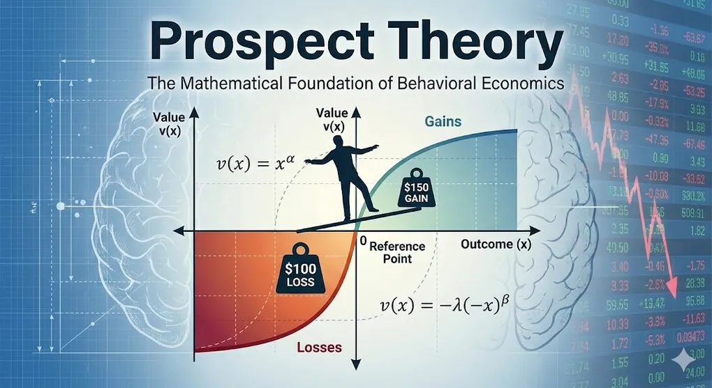
Prospect Theory: The Mathematical Foundation of Behavioral Economics

Behavioral Economics Prospect Theory Psychology Finance Python

The Theory That Won a Nobel Prize

In 1979, psychologists Daniel Kahneman and Amos Tversky published a paper that would revolutionize economics: “Prospect Theory: An Analysis of Decision under Risk.”

Their insight? Humans don’t evaluate outcomes rationally. We don’t calculate expected utility like economists assumed. Instead, we use mental shortcuts that lead to predictable irrationality.

“Losses loom larger than gains.”
— Kahneman & Tversky, 1979

This single sentence captures decades of research and earned Kahneman the 2002 Nobel Prize in Economics.

The Problem with Expected Utility Theory

Traditional economics relies on Expected Utility Theory (EUT):

Expected Value = Σ (Probability × Outcome)

Under EUT, a rational person evaluating a bet would:

Calculate the probability-weighted value of each outcome
Choose the option with the highest expected value

But humans don’t behave this way.

EUT Prediction	What People Actually Do
Accept any positive expected value bet	Reject many favorable bets
Treat $100 gained =$ 100 lost	Feel losses ~2x more intensely
Evaluate outcomes independently	Compare to a reference point

The Value Function: An S-Curve

The heart of Prospect Theory is the value function—a mathematical representation of how we perceive gains and losses.

Three Key Properties

Property	Description	Implication
Reference Dependence	Value is measured relative to a reference point, not absolute wealth	Same outcome feels different depending on expectations
Diminishing Sensitivity	The curve flattens as magnitude increases	$100→$ 200 feels bigger than $10,100→$ 10,200
Loss Aversion	The curve is steeper for losses than gains	Losing $100 hurts more than gaining$ 100 feels good

The Mathematical Formula

Kahneman and Tversky proposed this functional form:

v(x) = \begin{cases} x^\alpha & \text{if } x \ge 0 \text{ (gains)} \\ -\lambda(-x)^\beta & \text{if } x < 0 \text{ (losses)} \end{cases}

Where:

$\alpha, \beta \approx 0.88$ (diminishing sensitivity parameter)
$\lambda \approx 2.25$ (loss aversion coefficient)

Visualizing the Value Function

Here’s Python code to plot the classic S-curve:

import numpy as np
import matplotlib.pyplot as plt

def prospect_value(x, alpha=0.88, beta=0.88, lambda_=2.25):
    """
    Calculate subjective value according to Prospect Theory.
    
    Parameters:
    - x: outcome (gain if positive, loss if negative)
    - alpha: diminishing sensitivity for gains (default: 0.88)
    - beta: diminishing sensitivity for losses (default: 0.88)
    - lambda_: loss aversion coefficient (default: 2.25)
    """
    if x >= 0:
        return x ** alpha
    else:
        return -lambda_ * ((-x) ** beta)

# Generate data points
x = np.linspace(-100, 100, 1000)
v = [prospect_value(xi) for xi in x]

# Create the plot
fig, ax = plt.subplots(figsize=(10, 8))

# Plot the value function
ax.plot(x, v, 'b-', linewidth=2.5, label='Value Function v(x)')

# Add reference lines
ax.axhline(y=0, color='gray', linestyle='-', linewidth=0.5)
ax.axvline(x=0, color='gray', linestyle='-', linewidth=0.5)

# Highlight key regions
ax.fill_between(x[x >= 0], 0, [prospect_value(xi) for xi in x[x >= 0]], 
                alpha=0.2, color='green', label='Gains (concave)')
ax.fill_between(x[x < 0], 0, [prospect_value(xi) for xi in x[x < 0]], 
                alpha=0.2, color='red', label='Losses (convex, steeper)')

# Annotations
ax.annotate('Reference Point', xy=(0, 0), xytext=(15, 30),
            fontsize=11, arrowprops=dict(arrowstyle='->', color='black'))
ax.annotate('Loss Aversion:\nSlope ~2.25x steeper', xy=(-50, prospect_value(-50)), 
            xytext=(-80, -100), fontsize=10,
            arrowprops=dict(arrowstyle='->', color='red'))
ax.annotate('Diminishing Sensitivity:\nCurve flattens', xy=(80, prospect_value(80)), 
            xytext=(60, 120), fontsize=10,
            arrowprops=dict(arrowstyle='->', color='green'))

# Labels and styling
ax.set_xlabel('Outcome (x)', fontsize=12)
ax.set_ylabel('Subjective Value v(x)', fontsize=12)
ax.set_title('Prospect Theory Value Function', fontsize=14, fontweight='bold')
ax.legend(loc='upper left')
ax.grid(True, alpha=0.3)

plt.tight_layout()
plt.savefig('prospect_theory_value_function.png', dpi=150, bbox_inches='tight')
plt.show()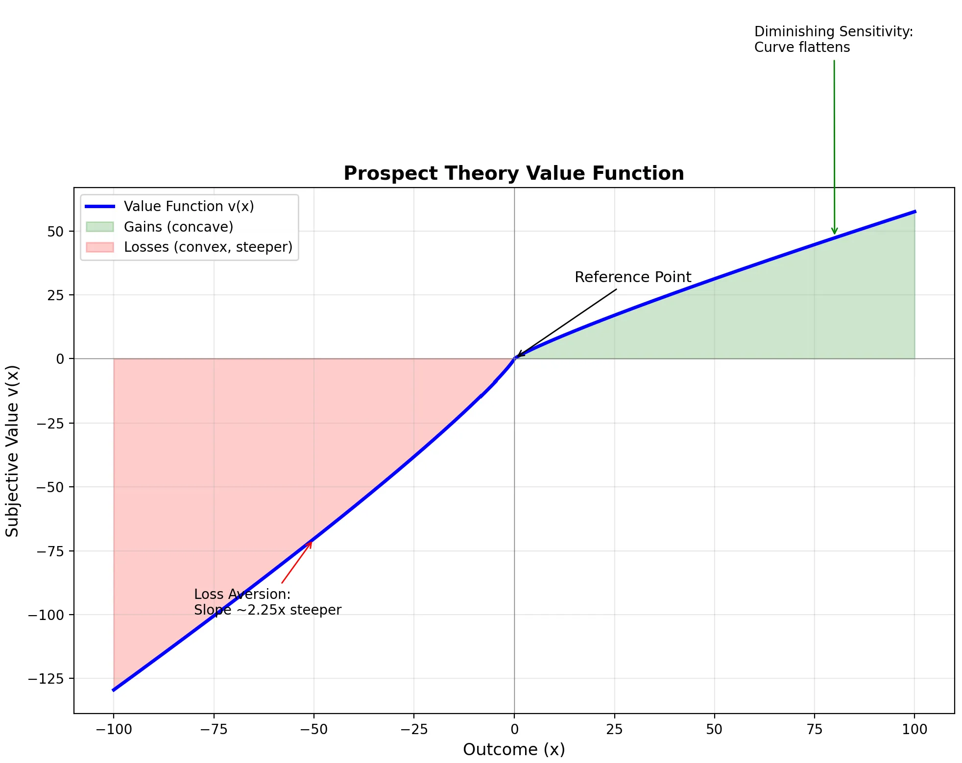

Prospect Theory Value Function - The classic S-curve showing loss aversion and diminishing sensitivity

What the Graph Reveals

Region	Shape	Behavior
Right of origin (Gains)	Concave (curves down)	Risk-averse for gains—prefer certain $50 over 50% chance of$ 100
Left of origin (Losses)	Convex (curves up)	Risk-seeking for losses—prefer 50% chance of losing $100 over certain$ 50 loss
Steepness comparison	Losses ~2.25x steeper	Same magnitude loss hurts more than gain feels good

Property 1: Reference Dependence

Our satisfaction depends not on absolute outcomes, but on comparisons to a reference point.

The Salary Paradox

Scenario	Objective Outcome	Subjective Experience
You get $100K bonus, colleagues get$ 50K	+$100K	😊 Thrilled
You get $100K bonus, colleagues get$ 200K	+$100K	😤 Disappointed

Same $100K. Completely different feelings. The reference point changed.

Practical Applications

Domain	Reference Point Manipulation
Pricing	Show “was $199, now$ 99” to set higher anchor
Negotiations	First offer becomes the reference
Performance Reviews	Compare to department average, not absolute metrics

Property 2: Diminishing Sensitivity

The value function is concave for gains and convex for losses. This means sensitivity decreases as you move away from the reference point.

The $100 Rule

Change	Subjective Impact
$0 →$ 100	HUGE
$1,000 →$ 1,100	Noticeable
$10,000 →$ 10,100	Barely register

This has profound implications for decision-making.

Strategic Application: Segregate Gains, Integrate Losses

Principle	Example
Segregate gains	Two $50 gifts feel better than one$ 100 gift
Integrate losses	One $100 loss hurts less than two$ 50 losses
Combine small loss with larger gain	” $100 off your$ 500 purchase” feels better than “$400 total”

UX Design Tip: Because of diminishing sensitivity, separating a painful process into smaller chunks doesn’t help—it might make it worse by resetting the reference point each time. But bundling “painful” payments into one single transaction (integration of losses) reduces total psychological pain.
This is why Amazon Prime works—one payment, zero shipping pain for the rest of the year.

Property 3: Loss Aversion (λ ≈ 2.25)

The most famous finding: losses hurt approximately 2.25 times more than equivalent gains feel good.

The Coin Flip Experiment

Would you accept this bet?

Heads: You win $150
Tails: You lose $100

Expected value: +$25. Most people reject this bet.

Why? The potential $100 loss looms larger than the$ 150 gain.

For most people, you need to offer around $200-$ 250 to win before they’ll risk losing $100.

Loss Aversion in Practice

Domain	Manifestation
Investing	Disposition effect—selling winners too early, holding losers too long
Endowment Effect	Owning something increases its perceived value
Status Quo Bias	Preference for current state (change = potential loss)
Risk Premiums	Stocks must offer higher returns to compensate for volatility

Advanced: Probability Weighting Function

Prospect Theory has a second component often overlooked: probability weighting.

We don’t perceive probabilities linearly either.

The Weighting Function

The probability weighting function $\pi(p)$ transforms objective probabilities into subjective decision weights:

\pi(p) = \frac{p^\gamma}{(p^\gamma + (1-p)^\gamma)^{1/\gamma}}

Where $\gamma \approx 0.61$ (curvature parameter from Tversky & Kahneman 1992).

Visualization Code:

import numpy as np
import matplotlib.pyplot as plt

def probability_weight(p, gamma=0.61):
    """
    Probability weighting function from Prospect Theory.
    
    Parameters:
    - p: objective probability (0 to 1)
    - gamma: curvature parameter (default: 0.61 from Tversky & Kahneman 1992)
    """
    return (p ** gamma) / ((p ** gamma + (1 - p) ** gamma) ** (1 / gamma))

# Visualize the probability weighting function
p = np.linspace(0.01, 0.99, 100)
w = [probability_weight(pi) for pi in p]

fig, ax = plt.subplots(figsize=(10, 8))

# Plot the weighting function
ax.plot(p, w, 'b-', linewidth=2.5, label='Probability Weight π(p)')

# Reference line (rational = linear)
ax.plot([0, 1], [0, 1], 'k--', linewidth=1, alpha=0.5, label='Rational (π(p) = p)')

# Highlight overweighting and underweighting regions
ax.fill_between(p[p < 0.35], [probability_weight(pi) for pi in p[p < 0.35]], p[p < 0.35], 
                where=[probability_weight(pi) > pi for pi in p[p < 0.35]],
                alpha=0.3, color='orange', label='Overweighted (small p)')
ax.fill_between(p[p > 0.35], [probability_weight(pi) for pi in p[p > 0.35]], p[p > 0.35], 
                where=[probability_weight(pi) < pi for pi in p[p > 0.35]],
                alpha=0.3, color='purple', label='Underweighted (large p)')

# Annotations
ax.annotate('We overweight\nsmall probabilities\n→ Buy lottery tickets', 
            xy=(0.05, probability_weight(0.05)), xytext=(0.15, 0.35),
            fontsize=10, arrowprops=dict(arrowstyle='->', color='orange'))
ax.annotate('We underweight\nlarge probabilities\n→ Buy insurance', 
            xy=(0.95, probability_weight(0.95)), xytext=(0.65, 0.7),
            fontsize=10, arrowprops=dict(arrowstyle='->', color='purple'))

# Labels
ax.set_xlabel('Objective Probability (p)', fontsize=12)
ax.set_ylabel('Decision Weight π(p)', fontsize=12)
ax.set_title('Probability Weighting Function (Inverse S-Curve)', fontsize=14, fontweight='bold')
ax.legend(loc='upper left')
ax.grid(True, alpha=0.3)
ax.set_xlim(0, 1)
ax.set_ylim(0, 1)

plt.tight_layout()
plt.savefig('probability_weighting_function.png', dpi=150, bbox_inches='tight')
plt.show()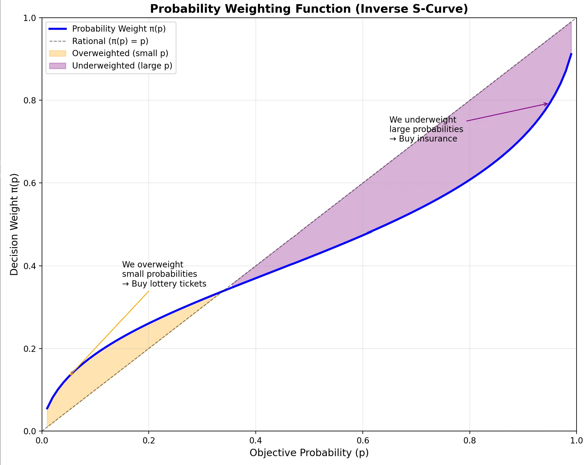

Probability Weighting Function - The inverse S-curve showing overweighting of small probabilities and underweighting of large probabilities

Key Distortions

Objective Probability	Subjective Weight	Implication
Very small (0.1%)	Overweighted	We buy lottery tickets
Very large (99.9%)	Underweighted	We buy insurance
Moderate (40-60%)	Roughly accurate	Less distortion in middle

Why We Buy Both Lottery Tickets AND Insurance

This seems contradictory:

Lottery: Negative expected value, but we pay anyway
Insurance: Often negative expected value, but we pay anyway

Prospect Theory explains both:

Lottery: Overweight tiny probability of huge gain
Insurance: Overweight tiny probability of catastrophic loss

The Fourfold Pattern of Risk Attitudes

Kahneman’s famous table explains how probability weighting + value function create four distinct behavioral modes:

Probability	Gains	Losses
High (95%)	🔒 Risk Averse	🎲 Risk Seeking
	Fear of disappointment	Hope to avoid loss
	Accept unfavorable settlement	Reject favorable settlement
	”Take the sure $900 vs. 95% of$ 1000"	"Gamble to avoid $900 loss”
Low (5%)	🎲 Risk Seeking	🔒 Risk Averse
	Hope of large gain	Fear of large loss
	Buy lottery tickets	Buy insurance
	”5% chance at $10,000? I’m in!"	"What if disaster strikes? I’ll pay.”

Key Insight: The same person can be risk-seeking AND risk-averse—depending on whether they’re facing gains vs. losses and high vs. low probability. This is the Fourfold Pattern.

Detecting Prospect Theory in Data

As a data analyst, you can identify Prospect Theory effects in behavioral data:

1. Asymmetric Response to Gains vs. Losses

# Compare user reaction to equivalent gains and losses
def detect_loss_aversion(df):
    """
    Detect loss aversion in user behavior data.
    
    Expects columns: 'outcome_change', 'user_action_intensity'
    """
    gains = df[df['outcome_change'] > 0]
    losses = df[df['outcome_change'] < 0]
    
    avg_gain_response = gains['user_action_intensity'].mean()
    avg_loss_response = losses['user_action_intensity'].abs().mean()
    
    loss_aversion_ratio = avg_loss_response / avg_gain_response
    
    print(f"Loss Aversion Ratio: {loss_aversion_ratio:.2f}")
    print(f"(Prospect Theory predicts ~2.25)")
    
    return loss_aversion_ratio

2. Reference Point Detection

Look for discontinuities at round numbers or historical benchmarks:

Stock behavior around $100 price points
Conversion rates around competitor pricing
Performance changes around last year’s metrics

3. Diminishing Sensitivity Curves

Plot response intensity against outcome magnitude—look for the S-curve pattern.

Summary: The Complete Prospect Theory Framework

Component	Formula	Key Insight
Value Function	$v(x) = x^{0.88}$ (gains), $-2.25 \cdot \\|x\\|^{0.88}$ (losses)	Asymmetric S-curve
Reference Dependence	$v(x)$ evaluated relative to $r$	Context matters more than absolute value
Diminishing Sensitivity	Concave gains, convex losses	Marginal impact decreases
Loss Aversion	$\lambda \approx 2.25$	Losses hurt 2x more than gains feel good
Probability Weighting	$\pi(p)$ overweights extremes	Small probabilities feel larger