OLTP vs. OLAP: A Deep Dive into Data Architecture
“The first time I ran an OLAP query on a production database, the website crashed for 5 minutes. That day, I learned why we strictly separate these two worlds.”
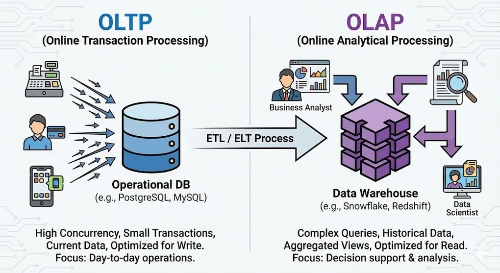
In the world of data engineering, the “One size fits all” approach is the biggest myth. The reason we strictly separate OLTP (Online Transaction Processing) and OLAP (Online Analytical Processing) systems lies in a fundamental trade-off in computer science: the physical difference between optimizing for Writes versus optimizing for Reads.
This article goes beyond surface-level definitions to explore the business logic, underlying storage structures, and data modeling strategies that differentiate these two pillars of data architecture.
1. Core Definitions & Business Context
OLTP: Online Transaction Processing
OLTP systems are the heartbeat of business operations, designed to capture events the moment they occur.
- Keywords: Atomicity, High Concurrency, Real-time, Low Latency.
- Business Focus:
- Micro View: Focuses on single entities (e.g., one customer, one specific order, one payment).
- Mission-Critical: If the system goes down, the business stops immediately (e.g., an ATM rejecting cards).
- Typical Operations: High volume of
INSERT,UPDATE,DELETE, and simple point-lookups.
Example OLTP Query (Point Lookup):
-- Fast: Uses Primary Key index, returns in milliseconds
SELECT order_id, status, total_amount, created_at
FROM orders
WHERE order_id = 12345;

-- Typical write operation
INSERT INTO orders (user_id, product_id, quantity, total_amount)
VALUES (789, 456, 2, 59.99);
The Backend Perspective: Scaling OLTP
Before we even talk about analytics, backend engineers face their own set of data challenges just to keep the application running. This is the “Data Management Approach” phase.
The Monolith: When your system is small, you have one application and one database. Simple.
Database per Service: As the system grows into Microservices (e.g., Order Service, Inventory Service), you split the monolith. Now, each service owns its private database to ensure loose coupling.
The Consistency Challenge: To keep data in sync across these services without a shared database, you implement patterns like Saga to manage distributed transactions.
The Goal here: Speed and Stability. At this stage, your entire focus is: “Make the App run fast, don’t let it crash.” This is pure OLTP. But once your manager asks, “How did our inventory levels correlate with sales across all services last year?”, your Microservices architecture hits a wall. That is where OLAP begins.
OLAP: Online Analytical Processing
OLAP systems are the brain of the business, responsible for transforming accumulated data into actionable insights.
- Keywords: Aggregation, High Throughput, Multidimensional, Historical.
- Business Focus:
- Macro View: Focuses on trends, group behaviors, and historical comparisons.
- Decision Support: If the system goes down, immediate sales aren’t stopped, but strategic decision-making pauses.
- Typical Operations: Complex
SELECTqueries involving heavy aggregations.
Example OLAP Query (Aggregation):
-- Slow on OLTP, Fast on OLAP: Scans millions of rows
SELECT
    DATE_TRUNC('month', order_date) AS month,
    p.category,
    SUM(f.amount) AS total_sales,
    COUNT(DISTINCT f.user_id) AS unique_customers,
    AVG(f.amount) AS avg_order_value
FROM fact_sales f
JOIN dim_product p ON f.product_id = p.product_id
JOIN dim_time t ON f.time_id = t.time_id
WHERE t.year = 2024
GROUP BY 1, 2
ORDER BY total_sales DESC
LIMIT 20;
2. Under the Hood: Storage Engines
This is the dividing line between a junior and a senior understanding. The physical layout of data on the disk dictates the system’s capabilities.
Row-Oriented vs. Column-Oriented
graph LR
    subgraph "Row-Oriented (OLTP)"
        R1["Row 1: ID=1, Name=Alice, Age=25, City=NYC"]
        R2["Row 2: ID=2, Name=Bob, Age=30, City=LA"]
        R3["Row 3: ID=3, Name=Carol, Age=28, City=SF"]
        R1 --> R2 --> R3
    end

    subgraph "Column-Oriented (OLAP)"
        C1["ID Column: 1, 2, 3"]
        C2["Name Column: Alice, Bob, Carol"]
        C3["Age Column: 25, 30, 28"]
        C4["City Column: NYC, LA, SF"]
end| Feature | OLTP (Row-Oriented) | OLAP (Column-Oriented) |
|---|---|---|
| Physical Storage | Data stored row by row | Data stored column by column |
| I/O Pattern | Fast Point-Reads: One disk seek for full row | Fast Analytics: Only reads needed columns |
| Compression | Low: Mixed data types per row | High (10:1+): Similar values compress well |
| Tech Stack | MySQL, PostgreSQL, SQL Server | Snowflake, BigQuery, ClickHouse |
Why Column Storage Wins for Analytics
When calculating AVG(Age) across 1 million users:
- Row Storage: Must read all columns (ID, Name, Age, City, …) = ~100MB I/O
- Column Storage: Only reads Age column = ~4MB I/O (96% reduction!)
3. Indexing Strategies
OLTP: B-Tree Index
- Structure: Balanced tree optimized for point lookups and range scans
- Best for:
WHERE id = 123orWHERE date BETWEEN x AND y - Trade-off: Every
INSERTmust update the index
OLAP: Bitmap Index & Zone Maps
- Bitmap Index: Efficient for low-cardinality columns (e.g., Status: Active/Inactive)
- Zone Maps: Metadata that stores min/max per data block, enabling “skip scan”
- Best for:
WHERE status = 'COMPLETED'across billions of rows
4. Data Modeling Strategies
OLTP: Normalization (3NF)
- Goal: Eliminate Data Redundancy to ensure data integrity.
- Structure: Data is fragmented across dozens of related tables.
- Trade-off: Queries require many
JOINs, which is computationally expensive for analytics.
OLAP: Dimensional Modeling (Star Schema)
erDiagram
    FACT_SALES ||--o{ DIM_PRODUCT : "product_id"
    FACT_SALES ||--o{ DIM_TIME : "time_id"
    FACT_SALES ||--o{ DIM_CUSTOMER : "customer_id"
    FACT_SALES ||--o{ DIM_STORE : "store_id"

    FACT_SALES {
        int sale_id PK
        int product_id FK
        int time_id FK
        int customer_id FK
        int store_id FK
        decimal amount
        int quantity
    }

    DIM_PRODUCT {
        int product_id PK
        string name
        string category
        string brand
    }

    DIM_TIME {
        int time_id PK
        date full_date
        int year
        int month
        string quarter
}- Goal: Optimize for Read Performance and analyst readability.
- Trade-off: Denormalization increases storage size and makes updates complex, but read speeds are blazing fast.
5. Scaling Strategies: Partitioning vs. Sharding
As data grows from gigabytes to petabytes, a single table (or even a single server) becomes a bottleneck. How we solve this depends heavily on whether we are optimizing for Writes (OLTP) or Reads (OLAP).
The OLAP Strategy: Partitioning (Divide & Conquer)
Partitioning splits a large table into smaller, manageable physical files based on a specific column key. The goal is Partition Pruning: allowing the query engine to completely ignore data that isn’t relevant to the query.
Common Partitioning Strategies:
-
Range Partitioning (The OLAP Standard):
- Logic: Data is split by a continuous range of values, most commonly Time.
- Use Case: “Store Jan 2024 data in File A, Feb 2024 in File B.”
- Benefit: Perfect for queries like
WHERE date BETWEEN '2024-01-01' AND '2024-02-01'.
-
List Partitioning:
- Logic: Data is split by discrete categorical values.
- Use Case: “US data in Partition 1, EU data in Partition 2.”
- Benefit: Ideal for multi-tenant architectures where queries always filter by
regionororg_id.
-
Hash Partitioning:
- Logic: A hash function is applied to a key (e.g.,
user_id) to distribute rows evenly across a fixed number of buckets. - Use Case: Preventing Data Skew. If “User A” has 1 million rows and “User B” has 10 rows, Range partitioning might create uneven file sizes. Hash ensures even distribution.
- Logic: A hash function is applied to a key (e.g.,
Benefits:
- Query scans only relevant partitions (partition pruning)
- Easier data lifecycle management (drop old partitions)
- Better compression within similar time ranges
-- BigQuery Example: Combining Range (Date) and Clustering (Sort Order)
CREATE TABLE sales_partitioned
PARTITION BY DATE(order_date) -- Physical split by day
CLUSTER BY product_category  -- Sorts data inside the partition
AS SELECT * FROM sales;
-- IMPACT:
-- A query for "Electronics in Jan 2024" will:
-- 1. PRUNE: Skip all partitions except Jan 2024 (saving TBs of scan).
-- 2. SEEK: Jump directly to 'Electronics' block inside that file.

-- This query only scans January 2024 partition (not entire table!)
SELECT SUM(amount)
FROM sales_partitioned
WHERE order_date BETWEEN '2024-01-01' AND '2024-01-31';
The OLTP Strategy: Sharding (Shared-Nothing)
While OLAP uses Partitioning to optimize reads, OLTP uses Sharding to optimize write throughput.
| Feature | Partitioning (OLAP focus) | Sharding (OLTP focus) |
|---|---|---|
| Concept | Logical split within one system | Physical split across different servers |
| Goal | Reduce I/O Scan Cost (Read Efficiency) | Distribute Write Load & Connections |
| Complexity | Low (Managed by DB engine) | High (App needs to know which shard to query) |
| Example | BigQuery Date Partitioning | User IDs 1-1M on DB Server A, User IDs 1M-2M on DB Server B |
Architectural Note: In modern Cloud Data Warehouses (Snowflake, BigQuery), “Sharding” is handled automatically under the hood (Compute separation). However, in the OLTP world (e.g., scaling PostgreSQL), Sharding remains a complex manual architecture decision often implemented at the application layer.
6. Performance Metrics & Trade-offs
OLTP: ACID & Latency
- ACID Compliance: Atomicity, Consistency, Isolation, Durability. Non-negotiable for financial data.
- Target: 99.9% of queries must complete in milliseconds.
- Bottleneck: Usually Lock Contention and Random I/O.
OLAP: Throughput & Scalability
- BASE Model: Basically Available, Soft state, Eventual consistency.
- Target: Scan Terabytes of data in seconds or minutes.
- Bottleneck: Usually Network Bandwidth and CPU/Memory for decompression.
7. The Architecture: ETL/ELT Pipeline
flowchart LR
    subgraph Sources
        A[(PostgreSQL<br/>OLTP)]
        B[(MySQL<br/>OLTP)]
        C[APIs]
    end

    subgraph Ingestion
        D[CDC / Debezium]
        E[Batch Jobs]
    end

    subgraph Transform
        F[dbt / Spark<br/>3NF → Star Schema]
    end

    subgraph Destination
        G[(Data Warehouse<br/>OLAP)]
    end

    subgraph Consume
        H[Power BI]
        I[Tableau]
        J[Python/R]
    end

    A --> D
    B --> E
    C --> E
    D --> F
    E --> F
    F --> G
    G --> H
    G --> I
G --> J- Source (OLTP): Application generates raw data (e.g., PostgreSQL).
- Ingestion: Data is extracted via CDC (Change Data Capture) or batch jobs.
- Transformation: Cleaning data & converting 3NF to Star Schema.
- Destination (OLAP): Data lands in the Data Warehouse for BI tools.
Pro Tip: Never attempt to run complex analytical queries on your OLTP production database. A heavy
SELECT *with aggregations can trigger table locks, freezing the application for actual users and causing a P0 incident. Yes, I learned this the hard way.
Summary
| Question | Answer |
|---|---|
| Building an App? | Use OLTP (PostgreSQL, MySQL) |
| Building a Dashboard? | Use OLAP (BigQuery, Snowflake) |
| Need both? | Set up an ETL/ELT pipeline between them |